The Mathematics of Societal Collapse: Implementing Structural-Demographic Theory

Mathematics is the language of patterns, and differential equations are the vocabulary for describing how things change. When Peter Turchin set out to create a science of history, he reached for the same mathematical tools that physicists use to describe planetary orbits and engineers use to design bridges. This was not an arbitrary choice. Differential equations have proven remarkably successful at capturing the dynamics of systems where many interacting components influence each other over time, from the flow of fluids to the oscillation of electrical circuits to the growth and decline of biological populations. If societies are systems in this technical sense, collections of interacting components whose behavior cannot be understood in isolation, then differential equations might be the right tool for modeling them. This essay explores that possibility in depth, explaining the mathematics that underlies Structural-Demographic Theory from first principles and documenting our implementation of these equations in Python.

The central insight that makes differential equations so powerful is deceptively simple: if you know how fast something is changing right now, you can figure out where it will be a moment from now. A car traveling at sixty miles per hour will be one mile down the road in one minute. But the real power emerges when the rate of change itself depends on the current state. A car that accelerates as it goes faster creates compound growth, with the change in position depending on the velocity, which itself depends on how long the car has been accelerating. Such systems can exhibit rich and sometimes surprising behavior, from steady growth to oscillations to chaos, all emerging from simple rules about how the rate of change depends on the current state.

The history of differential equations stretches back to the seventeenth century, when Isaac Newton and Gottfried Leibniz independently developed calculus, the mathematical framework for dealing with continuous change. Newton's motivation was physics: he wanted to describe the motion of planets under gravitational attraction. The position of a planet changes according to its velocity; the velocity changes according to the gravitational force; the gravitational force depends on position. This chain of dependencies, expressed mathematically, constitutes a differential equation. Newton's laws of motion, combined with his law of universal gravitation, allowed him to derive the elliptical orbits that Kepler had observed, a triumph of mathematical modeling that transformed our understanding of the cosmos.

The centuries since Newton have seen differential equations applied to an ever-widening range of phenomena. Heat conduction, fluid flow, electromagnetic waves, population ecology, chemical reactions, neural activity, economic dynamics, all can be modeled using differential equations. The specific equations differ, reflecting the different mechanisms at work in each domain, but the underlying mathematical structure is the same: rules specifying how the rate of change of some quantity depends on the current state of the system. This universality is both remarkable and useful. Techniques developed to solve one type of differential equation often work for others, and insights gained from studying one system can illuminate others.

To understand why this matters for studying societies, consider the simplest possible model of population growth. Suppose that each year, a certain fraction of the population has children, and a different fraction dies. If we denote the population at time t as N(t), then the change in population over a small time interval depends on the current population: more people means more births. The simplest mathematical expression of this idea is dN/dt = rN, where dN/dt represents the rate of change of population (the number of people added per unit time), and r is the net growth rate (births minus deaths per capita). This equation says that the population grows in proportion to its current size, a pattern known as exponential growth.

Exponential growth is mathematically elegant but biologically unrealistic. No population can grow forever without limit. Food runs out, disease spreads more easily in dense populations, and living space becomes scarce. The Belgian mathematician Pierre Francois Verhulst recognized this in the 1830s and proposed a modification that accounts for resource limitations. The logistic growth model captures this reality by modifying the simple exponential equation to include a carrying capacity, the maximum population that the environment can sustain. The modified equation is dN/dt = rN(1 - N/K), where K is the carrying capacity. When the population N is small compared to K, the term (1 - N/K) is close to 1, and the population grows nearly exponentially. But as N approaches K, this term approaches zero, and growth slows. If the population overshoots K, the term becomes negative, and the population declines. This simple modification produces dramatically different long-term behavior: instead of growing without bound, the population approaches and stabilizes at the carrying capacity.

The logistic equation illustrates a key concept that pervades the mathematics of complex systems: feedback. The growth rate of the population is not fixed; it depends on the population itself. When the population is low, the effective growth rate is high because resources are abundant. When the population is high, the effective growth rate is low or even negative because resources are strained. This negative feedback loop stabilizes the system, preventing runaway growth and maintaining the population near its carrying capacity. Positive feedback loops have the opposite effect: they amplify changes, driving the system away from equilibrium. A bank run, where fear of bank failure causes depositors to withdraw funds, which causes the bank to fail, which justifies the original fear, is an example of destabilizing positive feedback. Understanding feedback loops is essential to understanding Structural-Demographic Theory because the theory is built entirely on the interactions between variables that influence each other.

Now consider what happens when we add a second variable to our system. Suppose that the carrying capacity itself is not fixed but depends on another factor, say the level of technology. More advanced technology allows more food to be produced from the same land, effectively raising the carrying capacity. If we denote the technology level as T, we might write K = K_0 * T, where K_0 is some base carrying capacity and T measures technological advancement. If technology improves over time according to its own dynamics, perhaps at a rate that depends on the population size (more people means more potential inventors), then we have a system with two coupled equations: one for population and one for technology. The behavior of this system can be far more complex than either equation alone, with the two variables influencing each other in ways that produce dynamics neither would exhibit in isolation.

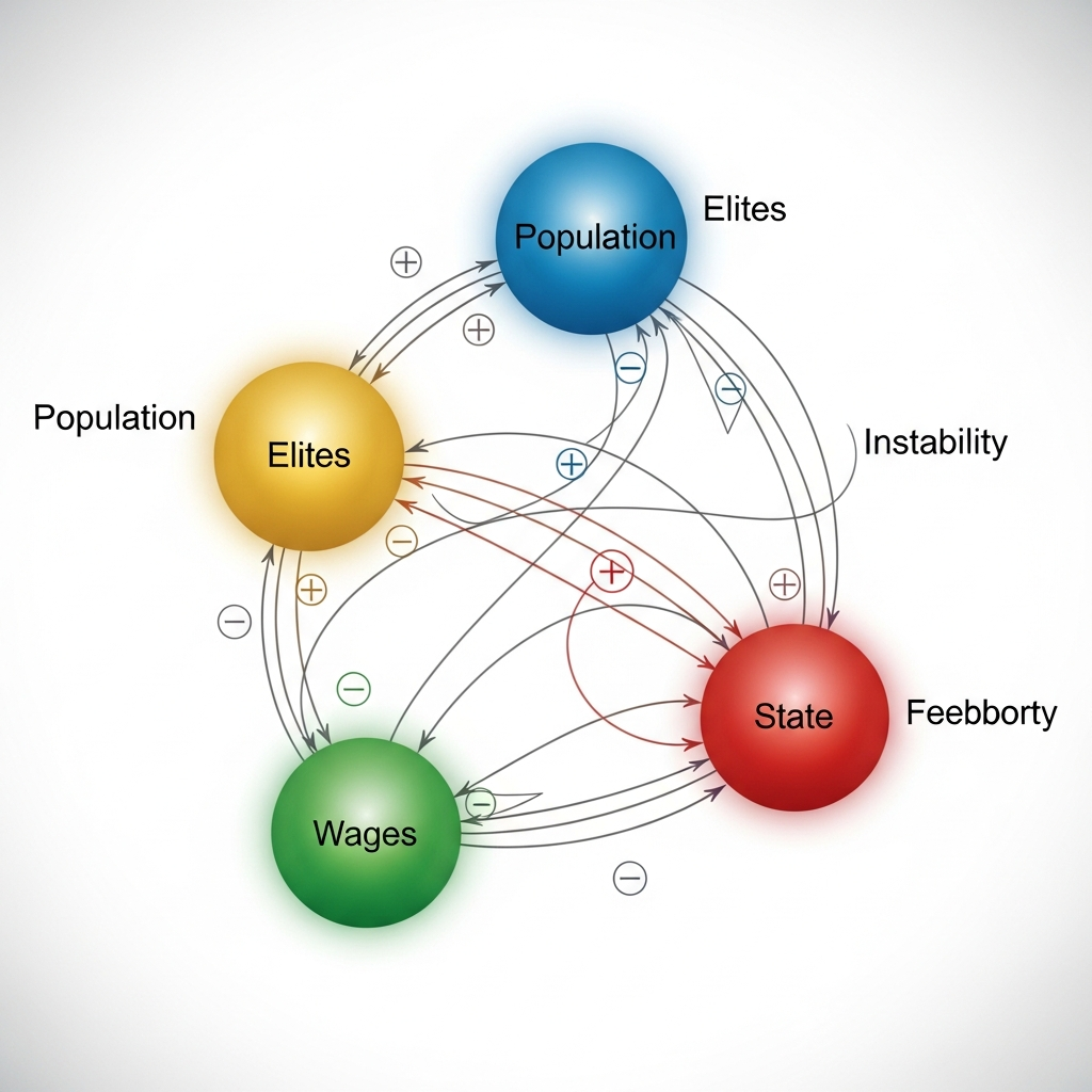
This is the essence of systems thinking: recognizing that the behavior of a complex whole emerges from the interactions among its parts. A society is not just a collection of individuals; it is a web of relationships, institutions, and processes that influence each other in intricate ways. Population affects labor supply, which affects wages, which affects birth rates, which affect population. Elites compete for positions, which strains state resources, which weakens the state's ability to maintain order, which creates opportunities for further elite competition. These chains of causation loop back on themselves, creating dynamics that cannot be predicted by studying any single variable in isolation.

The intellectual history of systems thinking in the social sciences is itself instructive. Early economists like Adam Smith and David Ricardo recognized that economic variables are interconnected, with prices, wages, profits, and rents all influencing each other. But they lacked the mathematical tools to formalize these relationships precisely. The marginalist revolution of the 1870s, led by William Stanley Jevons, Carl Menger, and Leon Walras, introduced calculus into economics, allowing for rigorous analysis of how markets reach equilibrium. General equilibrium theory, developed by Walras and perfected by Kenneth Arrow and Gerard Debreu in the twentieth century, showed how all markets in an economy can simultaneously clear, with supply equaling demand in every market. This was a mathematical tour de force, but it focused on static equilibrium rather than dynamic change. How economies move from one state to another, how they grow and contract and undergo crises, remained less well understood.

Sociology and political science developed their own traditions of systemic analysis, from Emile Durkheim's functionalism to Talcott Parsons's systems theory to Immanuel Wallerstein's world-systems theory. These approaches emphasized the interconnectedness of social phenomena and the way that institutions, norms, and power structures shape individual behavior. But they were largely qualitative, relying on verbal description and argument rather than mathematical formalization. The gap between these rich qualitative theories and the precision of mathematical modeling is what cliodynamics seeks to bridge.

Ordinary Differential Equations, commonly abbreviated as ODEs, are the mathematical framework for expressing these relationships precisely. The term "ordinary" distinguishes these equations from partial differential equations, which involve rates of change with respect to multiple independent variables (like both time and space). In cliodynamics, we typically work with ODEs where time is the only independent variable, and we track how multiple state variables evolve together over time. A system of ODEs consists of one equation for each state variable, with each equation specifying how that variable's rate of change depends on the current values of all the variables.

The five core equations of Structural-Demographic Theory form exactly such a system. The state variables are population (N), elite population (E), real wages or worker well-being (W), state fiscal health (S), and the Political Stress Index (psi, often written with the Greek letter). Each variable has its own equation describing how it changes over time, and each equation involves not just that variable but others in the system. The population equation, for instance, includes wages because better-fed populations grow faster. The elite equation includes both population (source of new elites) and wages (which affect surplus available for accumulation). The wage equation includes both population (labor supply) and elite numbers (which affect extraction). And so on. The result is a tightly coupled system where everything affects everything else.

Before diving into the specific equations, it is worth reflecting on why ODEs are suited to this kind of modeling. Historical dynamics unfold over time, with each moment building on what came before. The state of a society at any given time, its population, its class structure, its economic conditions, its political institutions, shapes what happens next. ODEs capture this temporal dependency naturally, expressing how the present state determines the direction and speed of change. They also capture the continuous nature of social processes. Population does not jump from one level to another overnight; it changes gradually as births and deaths accumulate. The same is true of wages, state finances, and political tensions. ODEs model these continuous changes using calculus, the mathematics of continuous change developed by Newton and Leibniz in the seventeenth century.

There is, of course, an important caveat. Real historical processes involve discrete events, random shocks, and discontinuous changes that ODEs handle poorly. Wars, plagues, assassinations, and natural disasters can abruptly alter a society's trajectory in ways that smooth differential equations cannot capture. The Black Death killed between one-third and one-half of Europe's population in a few years, a demographic shock far more rapid than any continuous process. Revolutions can overturn governments in days. Financial panics can collapse economies in weeks. These events matter enormously for the lived experience of history, and any complete account must grapple with them. Turchin's framework does not deny the importance of these events; rather, it seeks to understand the structural conditions that make societies more or less vulnerable to such shocks. A society with high political stress is like a forest during a drought: the specific spark that starts the fire matters less than the accumulated fuel that allows it to spread. ODEs model the accumulation of structural pressures, while recognizing that the specific events that trigger crises involve elements of chance that no mathematical model can fully predict.

With this conceptual foundation in place, let us turn to the specific equations of Structural-Demographic Theory. Our implementation follows the formulations in Turchin's Ages of Discord (2016) and Secular Cycles (2009, with Sergey Nefedov), translating the mathematical relationships described in those works into Python code that can be numerically solved. We will examine each equation in turn, explaining both the mathematical form and the historical intuition it encodes.

Population Dynamics: The Foundation of Society

Population is the foundation of any society. The number of people affects everything from labor supply to military strength to tax revenues. Demography, as Auguste Comte recognized, is destiny, at least in the sense that the size and composition of a population constrain what a society can accomplish. A society with ten million people can field larger armies, cultivate more land, and produce more goods than a society with one million. But it also faces greater challenges in coordination, resource distribution, and maintaining social cohesion. The relationship between population and prosperity is not straightforward; what matters is not just the number of people but their relationship to available resources and to each other.

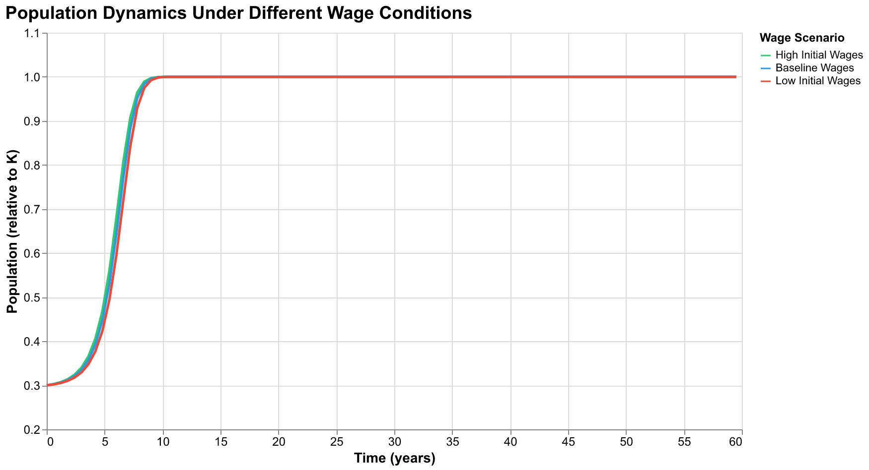
In Structural-Demographic Theory, population dynamics follow a modified logistic growth model where the growth rate depends on real wages. The equation is:

dN/dt = r(W) * N * (1 - N/K)

This looks like the standard logistic equation we discussed earlier, but with a crucial modification: the intrinsic growth rate r is not a constant but a function of wages W. Specifically, r(W) = r_max * (W/W_0)^beta, where r_max is the maximum possible growth rate when wages are at their baseline level W_0, and beta is a sensitivity parameter that controls how strongly wages affect growth. When wages equal the baseline W_0, the growth rate is r_max. When wages exceed the baseline, the growth rate is even higher. When wages fall below baseline, the growth rate drops, and if wages fall far enough, it can become negative (more deaths than births).

This wage-dependent growth rate captures what economists call the Malthusian mechanism, named after Thomas Malthus, the early nineteenth-century economist and clergyman who first articulated the relationship between population and resources in systematic terms. Malthus observed that population tends to grow geometrically (exponentially in modern terms) while food production grows only arithmetically (linearly). This mismatch, he argued, doomed most of humanity to perpetual poverty: any improvement in living standards would simply lead to population growth that returned living standards to subsistence level. When resources are abundant relative to population, people are well-fed, healthy, and able to raise more children. When resources are scarce, malnutrition, disease, and poverty reduce birth rates and increase death rates. The parameter beta controls the strength of this effect: higher values mean population responds more sensitively to economic conditions.

Historical evidence strongly supports the Malthusian mechanism for pre-industrial societies. Economic historians have documented the inverse relationship between population and real wages across many centuries and countries. Gregory Clark's seminal study of England from 1200 to 1800 showed that real wages were strongly correlated with population: when population was low (as after the Black Death), wages were high; when population recovered, wages fell. This pattern repeated across multiple cycles, suggesting a robust underlying mechanism. The Malthusian world was one where technological progress was slow relative to population growth, so any gains in productivity were quickly absorbed by additional people, returning living standards to subsistence.

The industrial revolution broke this Malthusian trap, at least for the countries that industrialized. Technological progress accelerated to the point where it outpaced population growth, allowing living standards to rise even as populations expanded. The carrying capacity, in effect, grew faster than the population pressing against it. But even in industrial economies, the relationship between population and wages does not entirely disappear. Labor markets still respond to supply and demand, and large increases in the working-age population can put downward pressure on wages. The baby boom generation's entry into the labor market in the 1970s coincided with the stagnation of wages that Turchin identifies as a key structural pressure in contemporary America. The Malthusian mechanism may be muted in modern economies, but it is not entirely absent.

In our Python implementation, the population dynamics function translates these concepts into code:

def population_dynamics(self, N: float, W: float, t: float) -> float:
    p = self.params
    r_effective = p.r_max * (W / p.W_0) ** p.beta
    dN_dt = r_effective * N * (1 - N / p.K_0)
    return dN_dt

The function takes the current population N, current wages W, and time t as inputs, and returns the rate of change of population. The time parameter t is not used in this autonomous system (the equations do not explicitly depend on time), but we include it for compatibility with standard ODE solver interfaces that expect functions of this signature. The calculation first computes the effective growth rate by adjusting the maximum rate r_max based on the wage ratio raised to the power beta, then applies the logistic growth formula.

The carrying capacity K_0 in this model represents the maximum population that can be sustained given the current level of technology and resource availability. Unlike some ecological models where carrying capacity varies dynamically with environmental conditions, our baseline implementation treats K_0 as a fixed parameter. This is a simplification; in reality, technological change, climate shifts, territorial expansion, and changes in social organization all alter the effective carrying capacity over time. Medieval Europe's carrying capacity expanded with the introduction of the heavy plow and the three-field rotation system. China's carrying capacity expanded with the introduction of American crops like maize and sweet potatoes in the early modern period. For analyzing secular cycles within a fixed technological regime, however, treating K_0 as constant is a reasonable approximation that greatly simplifies the mathematics without fundamentally distorting the dynamics.

Elite Dynamics: The Engine of Instability

If population is the foundation, elite dynamics are the engine that drives societal instability. Elites, those who hold or aspire to positions of power and prestige, compete for limited resources and positions. When the number of elites exceeds what the society can accommodate, this competition intensifies, generating the intra-elite conflict that Turchin identifies as the most reliable predictor of societal crisis.

The concept of elites requires careful definition. In everyday usage, the term often carries connotations of wealth, privilege, and perhaps illegitimate power. In Structural-Demographic Theory, the definition is more technical: elites are individuals who seek and expect positions of high status and influence, regardless of their current wealth or power. A law student expecting to become a partner at a prestigious firm is an aspiring elite, even if currently drowning in debt. A successful tradesperson earning a comfortable income but seeking nothing more is not, for the purposes of this analysis, part of the elite. What matters is the aspiration and expectation, not just the current condition.

This distinction matters because it is frustrated expectations, as much as actual deprivation, that generate political instability. A society where most people accept their station, where the ambitious can generally find satisfying positions, and where competition for power operates within established channels is stable even if inequality is high. A society where many ambitious individuals cannot find the status they believe they deserve, where competition becomes cutthroat and often violent, and where the establishment is seen as illegitimate by those it excludes is unstable even if absolute living standards are decent. Elite overproduction is dangerous precisely because it fills society with talented, ambitious, energetic people who have every incentive to challenge the existing order.

The equation governing elite population captures these dynamics:

dE/dt = alpha * f(surplus) * N - delta_e * E

This equation has two terms representing the inflows and outflows from the elite class. The first term models upward mobility: commoners becoming elites through wealth accumulation, educational credentials, political success, or other paths to status. The rate of upward mobility depends on the parameter alpha (the base mobility rate), a surplus factor that depends on economic conditions, and the total population N (the pool of potential aspirants). The second term models losses from the elite class through mortality and downward mobility (loss of status), at a rate delta_e per elite.

The surplus factor deserves careful explanation because it encodes a counterintuitive but historically important dynamic. When wages are high relative to the baseline, workers capture most of the economic output in the form of wages, leaving relatively little surplus for elite accumulation. When wages are low, the gap between total output and worker consumption is larger, providing more resources that can be captured by elites. We model this as f(surplus) = max(0, 1 - W/W_0 + mu), where mu is a parameter representing the baseline extraction rate that elites can achieve even when wages are at baseline levels. This formulation ensures that elite upward mobility increases when wages are depressed, which seems perverse from a welfare perspective but reflects historical reality. Periods of low wages are often periods of rapid elite expansion, as wealth concentrates at the top even as living standards fall for ordinary workers. The Gilded Age in America, the late Roman Republic, pre-revolutionary France, all combined wage stagnation for workers with rapid accumulation by the wealthy and explosive growth in the number of people seeking elite status.

The contrast between elite overproduction and elite scarcity illuminates the concept and its consequences. In a society with elite scarcity, there are more positions of power and prestige than qualified candidates to fill them. Think of frontier America, where vast territories needed governing, new businesses needed founding, and new institutions needed building. Such societies actively recruit ambitious individuals from lower strata, offering rapid advancement to those with talent and drive. Competition among elites is muted because opportunities are plentiful. The ruling class tends to be cohesive, united in defense of the existing order because that order serves their interests well, with little incentive to form factions or challenge the system that elevates them.

In a society with elite overproduction, the situation is reversed: more ambitious individuals than positions to accommodate them. Think of late imperial China, where the examination system produced far more qualified degree-holders than the bureaucracy could employ, creating a large class of frustrated scholars whose ambitions could find no legitimate outlet. Competition becomes fierce and often vicious. Factions form and vie for advantage, each seeking to advance its members at the expense of rivals. Those who cannot find positions within the establishment become critics of it, seeking to change the rules to their benefit or to overthrow the system entirely. The late Roman Republic offers a classic case study, with ambitious men like Marius, Sulla, Pompey, and Caesar turning to increasingly extreme measures, from proscriptions to civil war, in their competition for supremacy.

Our implementation captures these dynamics:

def elite_dynamics(self, E: float, N: float, W: float, t: float) -> float:
    p = self.params
    wage_ratio = W / p.W_0
    surplus_factor = max(0.0, 1.0 - wage_ratio + p.mu)
    upward_mobility = p.alpha * surplus_factor * N
    elite_loss = p.delta_e * E
    dE_dt = upward_mobility - elite_loss
    return dE_dt

Notice that upward mobility depends on the total population N. A larger population means more potential aspirants, more people with the talent and ambition to join the elite. This creates a positive feedback loop: population growth leads to more elites, which can lead to more competition and instability. But there is also a stabilizing mechanism: elite losses depend on the current elite population E. If elite numbers grow too large, losses through mortality and downward mobility also increase, eventually balancing the inflows. The tension between these opposing forces determines the equilibrium level of elite numbers and the oscillations around that equilibrium.

Wage Dynamics: The Pulse of the Economy

Real wages, a measure of purchasing power and living standards, respond to both labor market conditions and elite extraction. Wages are not just an economic variable; they are a summary statistic for the material well-being of ordinary people, the commoners who make up the vast majority of any society. When wages are high, people can afford better food, housing, and healthcare. They have time and energy for pursuits beyond mere survival. They can invest in their children's education and future. When wages are low, life is a struggle for survival, with little margin for error and little hope for improvement.

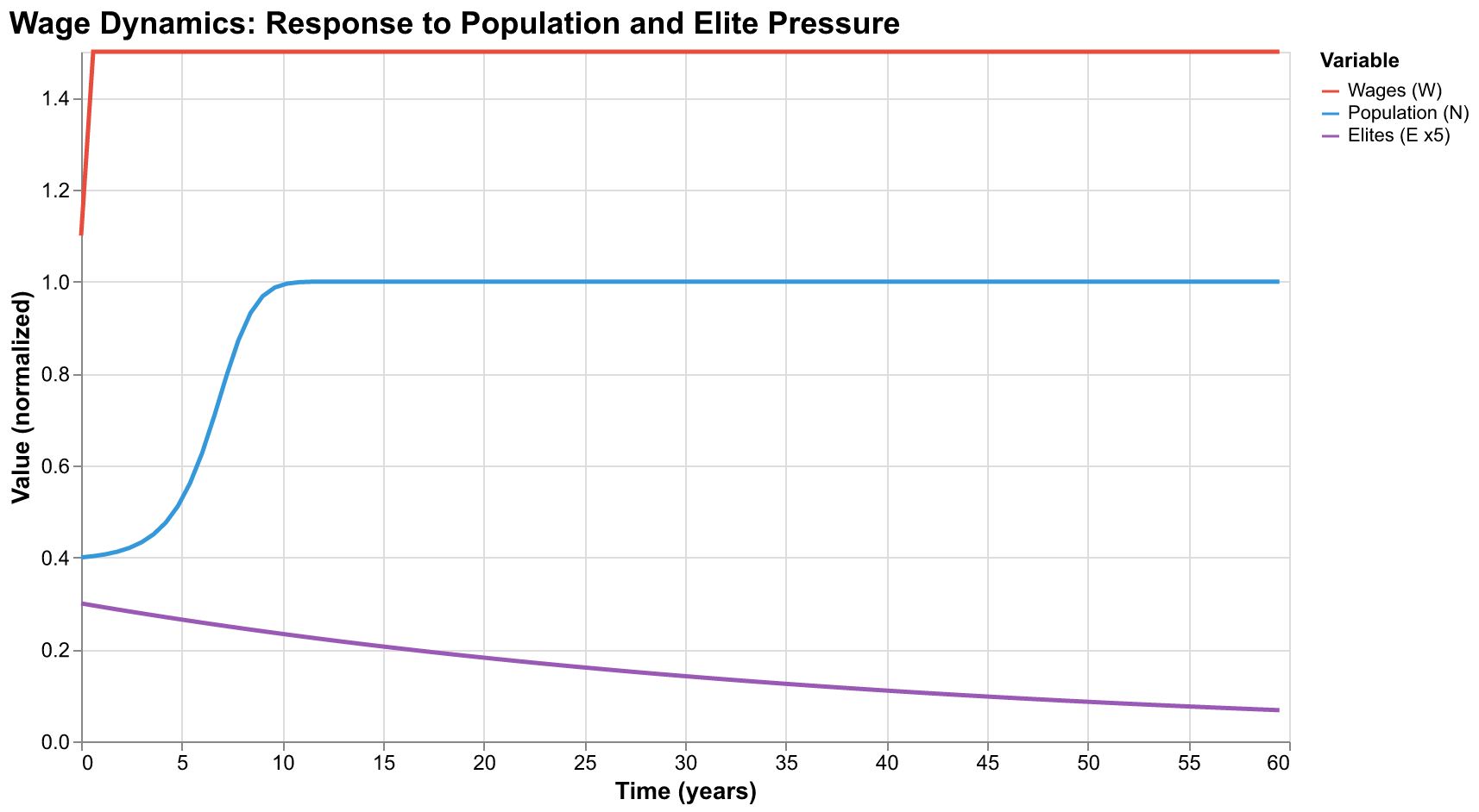
The equation governing wage dynamics captures two fundamental forces:

dW/dt = W * [gamma * (1 - N/K) - eta * (E/E_0 - 1)]

This equation has two components reflecting two forces that push wages in opposite directions. The first term, gamma * (1 - N/K), captures labor market tightness. The intuition is straightforward: when labor is scarce, employers must compete for workers, and wages rise. When labor is abundant, workers compete for jobs, and wages fall. The parameter gamma controls the strength of this effect, reflecting how responsive labor markets are to supply and demand imbalances.

When the population N is small relative to carrying capacity K, labor is scarce, the term (1 - N/K) is positive and large, and wages tend to rise. The aftermath of the Black Death in Europe illustrates this dramatically: with perhaps a third of the population dead, labor became extremely scarce, and wages for surviving workers rose substantially. Peasants could demand better terms from landlords; artisans could command higher prices for their work. This golden age for labor lasted until population recovered and the old pressures reasserted themselves.

When N approaches or exceeds K, labor is abundant, the term (1 - N/K) becomes small or negative, and downward pressure on wages increases. Workers compete for limited jobs, accepting lower pay rather than unemployment. The classic Marxist analysis of the "reserve army of labor" captures this dynamic: capitalists benefit from a pool of unemployed workers willing to undercut the wages of those currently employed, keeping wages near subsistence even as productivity rises.

The second term, eta * (E/E_0 - 1), captures elite extraction, a force that classical economics often neglects but that historical evidence suggests is crucial. When elite numbers E exceed the baseline E_0, more elites are competing for a share of economic output, and they extract more from workers through various mechanisms: higher rents, higher prices for goods and services controlled by elite-owned businesses, higher taxes to fund elite-captured government programs, and various forms of rent-seeking that transfer value from workers to elites without creating new wealth. The parameter eta controls the strength of this effect.

The extraction term operates through multiple channels in practice. Direct mechanisms include things like landlords raising rents, employers cutting benefits, and governments imposing regressive taxes. Indirect mechanisms include elite capture of regulatory processes that raise barriers to entry and reduce competition, financialization that extracts fees from economic transactions, and political influence that shapes laws in elite-friendly directions. The precise mechanisms vary across societies and historical periods, but the aggregate effect is similar: more elites competing for surplus means less for workers.

The multiplicative form W * [...] means that the rate of wage change is proportional to the current wage level. This ensures that wages change in percentage terms rather than absolute terms, which is economically sensible. A ten percent wage cut has the same significance whether wages start at one dollar or ten dollars. It also ensures that wages cannot become negative, since dW/dt = 0 when W = 0.

The distinction between popular immiseration and simple poverty is important for understanding the political consequences of wage dynamics. Poverty refers to an absolute condition: lacking the resources necessary for a decent life by some objective standard. Immiseration refers to a relative or temporal condition: deteriorating circumstances compared to the past or to expectations. A society can have low absolute poverty but high immiseration if living standards are falling from a previous peak. Post-World War II America achieved historically unprecedented prosperity for its working class; the stagnation since the 1970s represents immiseration relative to that benchmark, even though absolute living standards remain high by historical or global comparison.

It is immiseration, the perception of declining fortunes, that generates political discontent. People who have always been poor may accept their condition as natural or inevitable. People who expected to do better than their parents and find themselves falling behind are angry and seek someone to blame. The American Dream, the expectation that each generation will live better than the last, creates the psychological conditions for immiseration even at relatively high absolute living standards. When that dream fails, as it has for many Americans since the 1970s, the result is the political polarization and populist anger that characterizes our current moment.

def wage_dynamics(self, W: float, N: float, E: float, t: float) -> float:
    p = self.params
    labor_effect = p.gamma * (1 - N / p.K_0)
    elite_ratio = E / p.E_0
    extraction_effect = p.eta * (elite_ratio - 1)
    dW_dt = W * (labor_effect - extraction_effect)
    return dW_dt

State Dynamics: The Fiscal Health of Government

States require resources to function: to maintain armies, administer territories, provide public goods, and maintain legitimacy. The strength or weakness of the state is not merely a political variable; it is a structural feature that shapes what a society can accomplish collectively. A strong state can defend its borders, enforce contracts, build infrastructure, and provide the public goods that markets cannot efficiently supply. A weak state cannot do these things, leaving society vulnerable to external threats and internal disorder.

The equation for state fiscal health models the state as an entity with revenues and expenditures:

dS/dt = rho * Y - sigma * S - epsilon * E

Here Y represents economic output, which we model simply as W * N (wages times population, or the total wage bill, which is a rough proxy for the size of the economy). The term rho * Y is tax revenue: a fraction rho of economic output is collected by the state. In practice, this fraction varies enormously across societies and historical periods, from the light taxation of early modern England to the heavy extraction of command economies. But for any given society, there is typically a range within which taxation can operate without destroying the productive base, and the model captures the idea that revenues depend on the size of the economy.

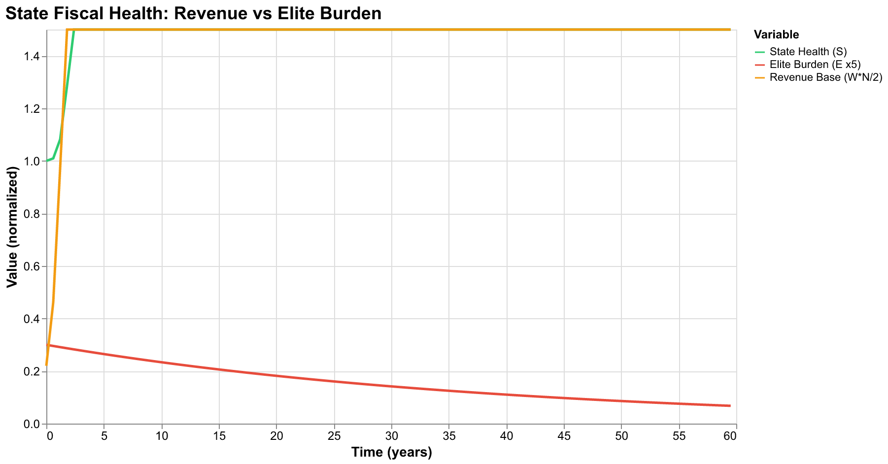
The term sigma * S is base expenditure: the state spends a fraction sigma of its accumulated resources on military, administration, and other ongoing functions. This captures the idea that states have fixed costs that must be met regardless of circumstances, and that these costs scale with the state's existing commitments. A larger state with more territory to defend, more bureaucrats to pay, and more obligations to meet has higher base expenditures than a smaller state.

The term epsilon * E is the elite burden: demands from elites for patronage, offices, and subsidies, which grow with elite numbers. This is where the political dynamics of elite overproduction connect to state fiscal health. Elites extract resources from the state in various ways: government jobs for their members, contracts for their businesses, subsidies for their projects, and favorable policies that transfer wealth in their direction. When elite numbers are moderate, these demands are manageable. When elite overproduction creates a surplus of ambitious individuals seeking resources, the demands exceed what the state can sustainably provide.

This equation captures a crucial dynamic: the state's fiscal health depends on the health of the broader economy and the demands placed upon it by elites. When wages are high (meaning Y = W * N is large) and elite numbers are moderate, revenues are strong and demands are manageable. The state can accumulate resources and maintain its functions effectively. It can invest in infrastructure, respond to challenges, and maintain the public goods that support prosperity. But when wages fall (reducing the tax base through lower W) and elite numbers rise (increasing demands through higher E), the state finds itself squeezed between declining revenues and rising expenditures.

This is the fiscal crisis that weakens states' ability to maintain order and respond to challenges. A state in fiscal crisis cannot invest in infrastructure, maintain its military, or provide the services its citizens expect. Its legitimacy erodes as it fails to meet obligations. Its officials become corrupt as they seek personal compensation for their declining institutional rewards. Its capacity to suppress conflict diminishes, allowing the tensions generated by elite overproduction and popular immiseration to explode into open disorder. The late Roman Empire, the late Ming Dynasty, the ancien regime in France, all exhibited this pattern of fiscal crisis preceding political collapse.

def state_dynamics(self, S: float, N: float, E: float, W: float, t: float) -> float:
    p = self.params
    output = W * N
    revenue = p.rho * output
    base_expenditure = p.sigma * S
    elite_burden = p.epsilon * E
    dS_dt = revenue - base_expenditure - elite_burden
    return dS_dt

The state dynamics equation is linear in the state variables, which makes it relatively well-behaved mathematically. The derivative depends linearly on S (through the base expenditure term) and E (through the elite burden term), and on the product W * N (through the revenue term). This linearity means the state equation by itself would have predictable exponential behavior. But its coupling to the other equations through W, N, and E means its behavior in the full system can still be complex. A state that starts healthy can be driven into crisis by the dynamics of population, elites, and wages acting through the system's feedback loops.

Instability Dynamics: The Political Stress Index

The Political Stress Index (PSI), denoted by the Greek letter psi, aggregates the structural drivers of instability into a single measure. While the previous four variables (N, E, W, S) can in principle be measured directly from historical or contemporary data, PSI is more abstract: it represents the accumulated potential for political disruption that the structural conditions have generated. High PSI does not mean that revolution is imminent tomorrow; it means that the kindling is dry and the matches are scattered about. A spark could set off a conflagration.

The equation governing PSI is:

dpsi/dt = lambda * [theta_w * (W_0/W - 1) + theta_e * (E/E_0 - 1) + theta_s * (S_0/S - 1)] - psi_decay * psi

Each of the three terms in brackets contributes positively to stress accumulation when conditions deteriorate. The first term, theta_w * (W_0/W - 1), measures popular immiseration: when wages W fall below the baseline W_0, the ratio W_0/W exceeds 1, the term becomes positive, and stress accumulates. The weight theta_w controls how strongly wage decline affects instability. The inverted form (W_0/W rather than W/W_0) means that a fifty percent wage decline contributes more stress than a fifty percent wage increase reduces it, capturing the asymmetry between losses and gains in psychological and political impact.

The second term, theta_e * (E/E_0 - 1), measures elite overproduction: when elite numbers E exceed the baseline E_0, this term is positive. The weight theta_e controls how strongly elite surplus affects instability. Elite overproduction matters because frustrated elites provide leadership, resources, and organization for political movements. A mass of discontented workers without elite leadership tends toward unfocused riots and protests. The same mass with elite leadership, with lawyers to draft manifestos, journalists to shape narratives, politicians to mobilize support, can become a revolutionary movement.

The third term, theta_s * (S_0/S - 1), measures state weakness: when state health S falls below baseline S_0, this term contributes to stress. Again, the inverted form captures the idea that state weakness is destabilizing: a state at half its baseline strength contributes significantly to stress, while a state at double its baseline strength does not proportionally reduce stress (there is limited benefit to having more state capacity than needed). The weight theta_s controls how strongly state weakness affects instability.

The parameter lambda controls the overall rate of stress accumulation. Higher values mean that structural pressures translate more quickly into elevated PSI. Lower values mean that pressures accumulate more slowly, giving societies more time to respond before reaching crisis levels. The decay term psi_decay * psi represents the natural dissipation of tensions when structural drivers are absent. Political stress is not permanent; grievances fade with time if not continually renewed. Social movements lose momentum if conditions improve. This decay ensures that PSI does not accumulate indefinitely but reaches some equilibrium determined by the balance between accumulation and decay.

def instability_dynamics(self, psi: float, E: float, W: float, S: float, t: float) -> float:
    p = self.params
    wage_stress = p.theta_w * max(0.0, p.W_0 / max(W, 1e-6) - 1)
    elite_stress = p.theta_e * max(0.0, E / p.E_0 - 1)
    state_stress = p.theta_s * max(0.0, p.S_0 / max(S, 1e-6) - 1)
    accumulation = p.lambda_psi * (wage_stress + elite_stress + state_stress)
    decay = p.psi_decay * psi
    dpsi_dt = accumulation - decay
    return dpsi_dt

Notice the use of max(0, ...) and max(W, 1e-6) in the implementation. These safeguards ensure numerical stability by preventing division by zero (if W or S somehow reached exactly zero) and keeping stress contributions non-negative (since improving conditions should reduce the accumulation rate to zero rather than create negative accumulation). These are the kinds of details that matter for robust implementation but that mathematical exposition often glosses over.

The Complete System: Coupling the Equations

The five equations described above form a coupled system of ordinary differential equations. To see how they work together, consider the following scenario: a society starts in a favorable condition with moderate population, few elites, high wages, strong state finances, and low political stress. What happens next?

With high wages, population grows toward the carrying capacity. This growth gradually increases labor supply, putting downward pressure on wages. As wages fall, surplus becomes available for elite accumulation, and elite numbers begin to rise. Rising elite numbers increase extraction from workers, further depressing wages. They also increase demands on the state, straining state finances. As wages fall, elite numbers rise, and state health declines, all three drivers of instability become active, and PSI begins to accumulate. The society is now on the path to crisis.

The complete system method combines all five equations:

def system(self, y: ArrayLike, t: float) -> NDArray[np.float64]:
    N, E, W, S, psi = y
    N = max(N, 1e-10)
    E = max(E, 1e-10)
    W = max(W, 1e-10)
    S = max(S, 1e-10)
    psi = max(psi, 0.0)

    dN_dt = self.population_dynamics(N, W, t)
    dE_dt = self.elite_dynamics(E, N, W, t)
    dW_dt = self.wage_dynamics(W, N, E, t)
    dS_dt = self.state_dynamics(S, N, E, W, t)
    dpsi_dt = self.instability_dynamics(psi, E, W, S, t)

    return np.array([dN_dt, dE_dt, dW_dt, dS_dt, dpsi_dt])

This system method is the interface that ODE solvers use to integrate the equations forward in time. Given a state vector y containing the current values of all five variables and a time t, it returns the derivatives, the rates of change of each variable. The solver uses these derivatives to step the system forward, computing new values at a slightly later time, then calls the system method again to get new derivatives, and repeats this process until reaching the desired end time.

The constraints ensuring positive values (the max functions) are essential for numerical stability. ODE solvers can sometimes produce small negative values due to numerical error, especially when a variable is close to zero. Allowing negative population, negative wages, or negative state health would cause downstream calculations to fail or produce nonsensical results. These safeguards prevent such problems while having negligible effect on the dynamics when variables are well above zero.

Why Analytical Solutions Do Not Exist

A natural question at this point is whether we can solve these equations analytically, finding formulas that express N(t), E(t), W(t), S(t), and psi(t) as explicit functions of time without needing numerical computation. The answer, for systems of this complexity, is almost always no, and understanding why illuminates important features of nonlinear dynamics.

Analytical solutions exist for a small class of differential equations, primarily those that are linear or that possess special mathematical structures that allow them to be transformed into solvable forms. Linear equations have the property that if y_1 and y_2 are solutions, then any linear combination a*y_1 + b*y_2 is also a solution. This superposition principle allows complex solutions to be built from simpler ones and leads to systematic solution methods. The differential equation for radioactive decay, dN/dt = -lambda*N, is linear and has the analytical solution N(t) = N_0 * exp(-lambda*t).

Some nonlinear equations can also be solved analytically if they have special properties. The logistic equation, dN/dt = rN(1 - N/K), is separable: it can be rearranged so that all terms involving N are on one side and all terms involving t are on the other. The solution is N(t) = K / (1 + (K/N_0 - 1) * exp(-rt)), a formula that gives the population at any time t given the initial population N_0. Separable equations, exact equations, and certain other classes have known solution techniques, but these classes are quite restricted compared to the full space of possible differential equations.

The SDT system is neither linear nor separable. The wage-dependent growth rate in the population equation couples population dynamics to the wage equation. The surplus factor in the elite equation couples elite dynamics to wages. The extraction term in the wage equation couples wages back to elite numbers. The revenue term in the state equation involves the product W*N. The instability equation involves ratios and inversions of multiple variables. These couplings create a web of dependencies that cannot be disentangled by the techniques that work for simpler equations.

This is not a limitation of our mathematical sophistication; it is a fundamental property of nonlinear coupled systems. Even apparently simple systems can have no analytical solutions. The Lorenz equations, discovered by meteorologist Edward Lorenz in 1963 while studying atmospheric convection, consist of just three equations with three parameters:

dx/dt = sigma * (y - x)

dy/dt = x * (rho - z) - y

dz/dt = x * y - beta * z

These equations are far simpler than SDT, yet their solutions can only be computed numerically. More remarkably, Lorenz discovered that these simple equations exhibit chaotic behavior: extreme sensitivity to initial conditions, such that tiny differences in starting points lead to completely different long-term trajectories. This sensitivity is often called the butterfly effect, from Lorenz's poetic suggestion that a butterfly flapping its wings in Brazil might trigger a tornado in Texas by creating a tiny perturbation that amplifies through the atmospheric dynamics.

The discovery that simple nonlinear equations could exhibit chaotic behavior was one of the great scientific surprises of the twentieth century. It challenged the Laplacian dream that perfect knowledge of the present would allow perfect prediction of the future. Even with perfect equations and arbitrarily precise measurements, chaotic systems are unpredictable beyond some time horizon because the inevitable small errors in measurement grow exponentially fast. This places fundamental limits on long-term prediction, not just practical limits from incomplete knowledge but theoretical limits from the mathematics of nonlinear dynamics.

The absence of analytical solutions is not a barrier to scientific understanding. Numerical methods allow us to compute solutions to arbitrary precision, explore the system's behavior across a wide range of parameters, and make predictions that can be tested against historical data. What we lose is the elegance of a closed-form formula that displays the solution's structure at a glance; what we gain is the ability to study systems complex enough to capture real-world phenomena. The trade-off is essential to progress in most areas of science and engineering.

Numerical Integration: How Computers Solve ODEs

Numerical integration is the process of computing approximate solutions to differential equations using discrete time steps. The basic idea is simple: start with the initial values of all variables at time t = 0, use the differential equations to compute how fast each variable is changing, use those rates of change to estimate where the variables will be a short time later, and repeat until reaching the desired end time. The challenge lies in doing this accurately and efficiently.

The simplest numerical method is Euler's method, named after the prolific eighteenth-century mathematician Leonhard Euler. Given the current state y at time t and the derivative dy/dt = f(y, t), the state at time t + h is approximately y + h * f(y, t), where h is the time step. This amounts to assuming that the rate of change is constant over the interval, which is accurate only if the interval is small enough that the derivative does not change much. Geometrically, Euler's method follows the tangent line from the current point for a small distance, then recomputes the tangent at the new point and follows it for another small distance, and so on.

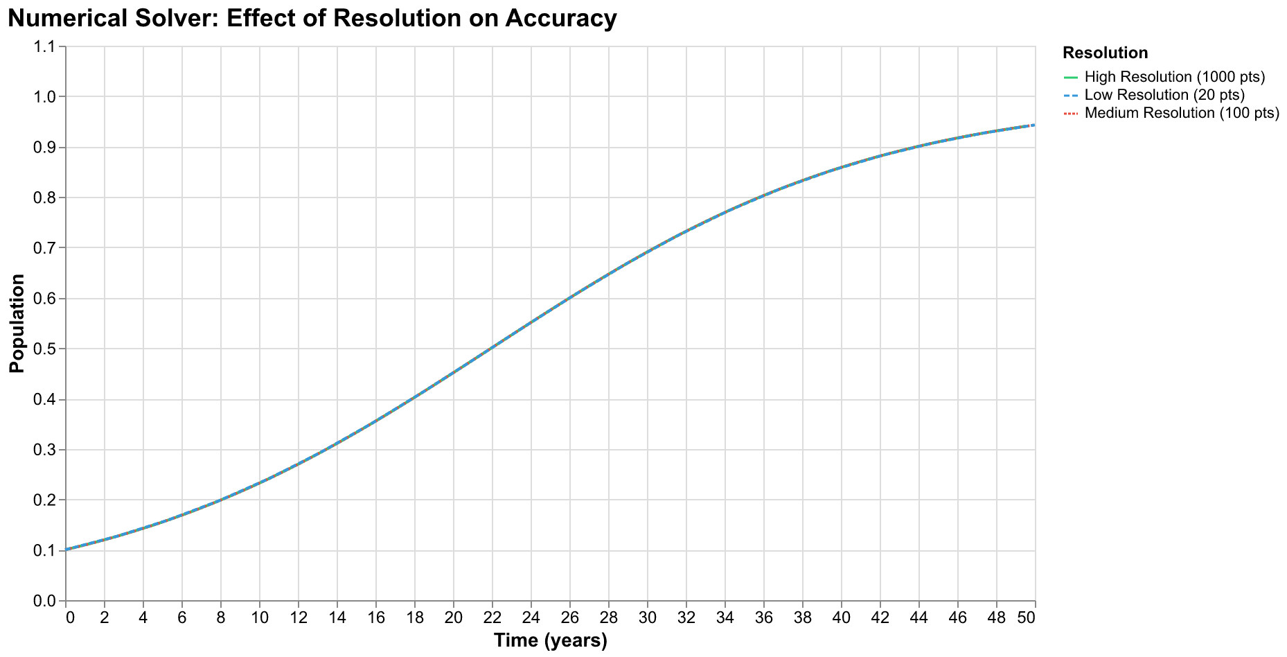
Euler's method is rarely used in practice because it requires very small time steps to achieve acceptable accuracy, making it computationally expensive for problems that span long time intervals. The error in each step is proportional to h^2, and these errors accumulate over many steps. Halving the step size reduces the error per step by a factor of four but doubles the number of steps needed, yielding only a factor of two improvement in total error. This unfavorable scaling makes Euler's method impractical for serious computation.

More sophisticated methods achieve better accuracy with larger time steps by using more information about how the derivative changes over the interval. The classic fourth-order Runge-Kutta method (RK4), developed around 1900, evaluates the derivative at multiple points within each interval: at the beginning, at the midpoint using an estimate from the beginning, at the midpoint again using a refined estimate, and at the end using the second midpoint estimate. These four evaluations are combined to estimate the change over the interval more accurately than any single evaluation could achieve. RK4 achieves fourth-order accuracy, meaning that the error per step is proportional to h^5, so the error decreases as the fourth power of the step size: halving the step size reduces the error by a factor of sixteen.

Modern ODE solvers typically use adaptive step size methods that automatically adjust the step size based on estimated local error. When the solution is changing rapidly, the solver takes smaller steps to maintain accuracy. When the solution is changing slowly, it takes larger steps to save computation. The solver estimates the error in each step by comparing the result from one method to the result from a slightly different method, and adjusts the step size to keep this estimated error within a specified tolerance.

The LSODA algorithm, available in scipy.integrate.odeint, is particularly sophisticated. It automatically detects whether the problem is "stiff" (having multiple timescales that differ greatly) and switches between methods optimized for stiff and non-stiff problems. Stiff problems are common in chemistry and biology, where some reactions proceed much faster than others, but can also arise in social dynamics when some processes equilibrate quickly while others evolve slowly. LSODA handles a wide range of equation types efficiently and adjusts step sizes adaptively, making it a good default choice for many applications.

Our implementation uses scipy's odeint function, which provides a convenient interface to LSODA:

from scipy.integrate import odeint
import numpy as np

# Create model with parameters
model = SDTModel(params)

# Initial state: [N, E, W, S, psi]
y0 = [0.5, 0.05, 1.0, 1.0, 0.0]

# Time points to compute solution
t = np.linspace(0, 200, 2000)  # 200 years, 2000 time points

# Integrate the system
solution = odeint(model.system, y0, t)

The result is a two-dimensional array where each row contains the values of all five variables at one time point. We can extract individual time series: solution[:, 0] gives population over time, solution[:, 1] gives elite population, and so on. These arrays can then be plotted, analyzed, or compared to historical data. The solver handles all the complexity of step size selection and error control internally, presenting a simple interface that takes a function defining the derivatives, an initial state, and a list of times at which to report the solution.

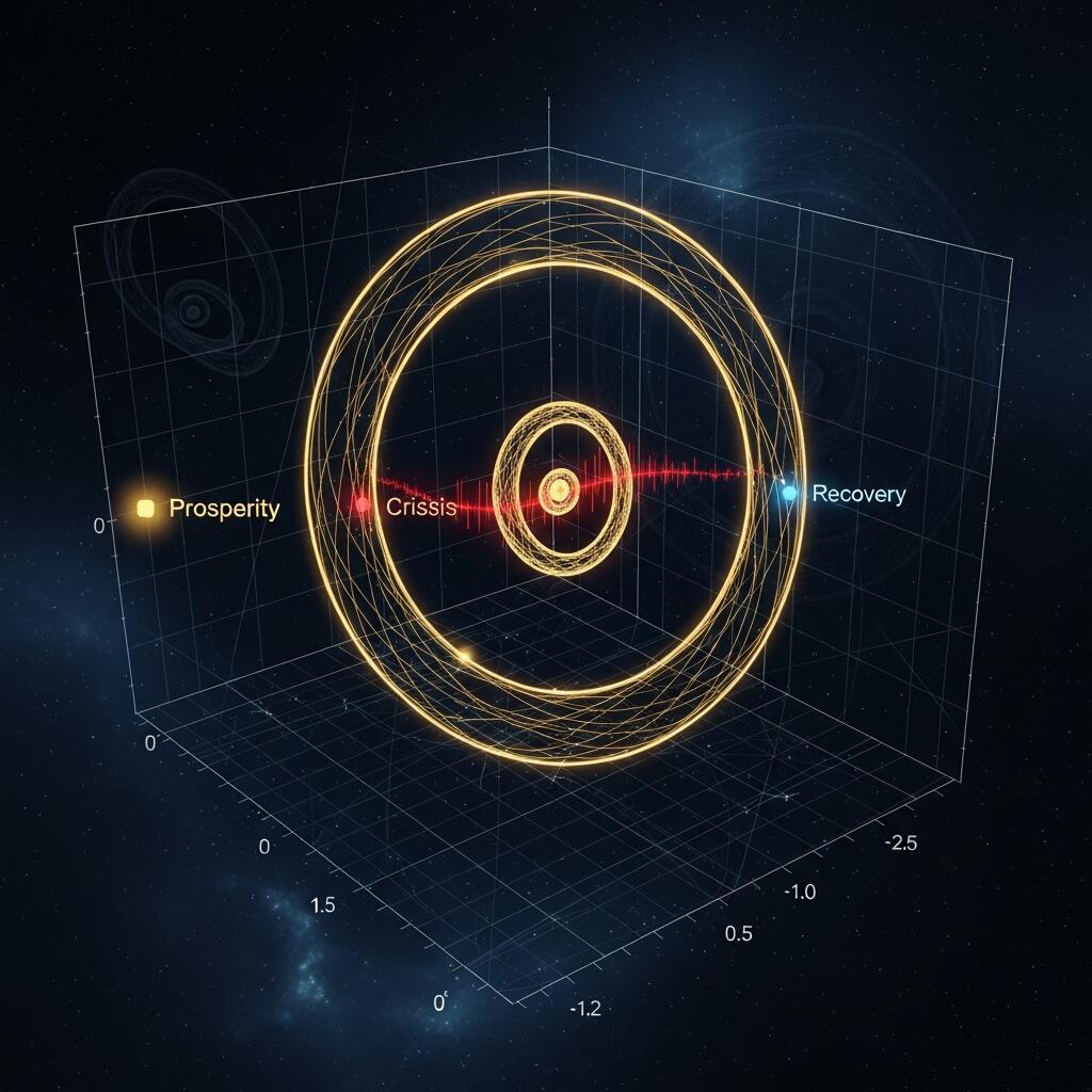
Phase Space: Seeing the Geometry of Change

One of the most powerful tools for understanding dynamical systems is phase space visualization. Phase space is an abstract mathematical space where each point represents a complete state of the system. For the SDT model, phase space is five-dimensional: each point is specified by a quintuple (N, E, W, S, psi) giving the values of all state variables. As the system evolves, it traces out a trajectory through this space, a curve that shows how the complete state changes over time.

Five dimensions cannot be directly visualized on a two-dimensional screen or page, but we can examine two-dimensional projections, slices through the full space that show how pairs of variables move together. A plot of E versus W, for example, shows how elite numbers and wages co-evolve. A plot of N versus psi shows how population and instability are related. Such projections can reveal important features of the dynamics: stable points where the system tends to settle, unstable points from which it tends to diverge, limit cycles where it oscillates periodically, and chaotic attractors where it wanders erratically but within bounded regions.

For the SDT system, phase portraits typically reveal oscillatory dynamics, consistent with the secular cycles that the theory predicts. The system does not settle to a fixed equilibrium where all derivatives are zero and nothing changes; rather, it traces out a closed or nearly closed loop in phase space, returning approximately to its starting region after a complete cycle. The period of this oscillation, the time it takes to complete one cycle, corresponds to the duration of the secular cycle, typically one to three centuries depending on parameter values.

The direction of motion around these cycles has a meaningful interpretation that connects the mathematics to historical intuition. In a typical cycle, population first rises while wages are still high (upper left region of a N-W plot). As population approaches carrying capacity, wages begin to fall (moving left). With depressed wages, elite numbers rise due to increased surplus available for accumulation (moving up in a E-W plot while continuing left). Rising elite extraction further depresses wages (continuing left). Eventually, some combination of factors, perhaps population decline from deteriorating conditions, elite losses from intensified competition, or reforms that reduce extraction, reverses the trends. Wages begin to recover, elite numbers stabilize and then decline, and the system begins a new cycle. The phase portrait shows this sequence geometrically, as a trajectory that spirals through the projections of the five-dimensional space.

Phase portraits also reveal the system's attractors, regions of phase space toward which trajectories tend to converge. A stable fixed point is an attractor that is a single point; trajectories starting nearby spiral inward and eventually come to rest there. A limit cycle is an attractor that is a closed curve; trajectories starting nearby approach the curve and then follow it indefinitely, oscillating forever with fixed period and amplitude. A chaotic attractor is a more complex object, often with a fractal structure, where trajectories are bounded but never repeat exactly, wandering erratically while remaining confined to a particular region.

The SDT system, for typical parameter values, appears to have a limit cycle attractor, consistent with the theory's prediction of recurring secular cycles. But the presence of multiple interacting variables and nonlinear couplings means that more complex dynamics are possible for some parameter ranges. Exploring this parameter space systematically is part of the scientific value of computational implementation: we can map out where different types of behavior occur and understand how parameter changes affect the qualitative character of the dynamics.

Sensitivity Analysis: How Parameters Shape Outcomes

A model is only as useful as the confidence we have in its predictions, and that confidence depends partly on understanding how sensitive the predictions are to the model's parameters. If small changes in parameter values lead to dramatically different outcomes, then uncertainty in those parameters translates to uncertainty in the predictions. If outcomes are robust to parameter changes, we can be more confident that the model's qualitative predictions will hold even if the parameter values are not precisely known.

Sensitivity analysis systematically explores how outcomes change as parameters vary. One approach is local sensitivity analysis: vary each parameter one at a time while holding others fixed, recording how the outcome of interest (such as the maximum PSI reached, or the period of the secular cycle, or the amplitude of wage oscillations) changes. This identifies which parameters most strongly influence each outcome, guiding where to focus calibration efforts and where parameter uncertainty matters most.

A more comprehensive approach is global sensitivity analysis, which varies all parameters simultaneously across their plausible ranges and uses statistical methods to decompose the variance in outcomes into contributions from each parameter and their interactions. Methods like Sobol indices quantify not just the main effect of each parameter but also how parameters interact, where the effect of one parameter depends on the values of others. Global sensitivity analysis is more computationally demanding but provides a more complete picture of how parameter uncertainty propagates through the model.

Our sensitivity analysis reveals that the SDT system's qualitative behavior, the existence of oscillatory cycles, is robust across a wide range of parameters. The specific period, amplitude, and phase of the cycles depend on parameter values, but cycles appear whenever the feedback loops are strong enough to create instability and the decay rates are not so high as to dampen oscillations immediately. This robustness is reassuring: it suggests that the theory captures genuine structural features of societal dynamics rather than artifacts of particular parameter choices.

Certain parameters have particularly strong effects on specific outcomes. The instability parameters (lambda_psi, the accumulation rate, and psi_decay, the decay rate) directly control the amplitude and persistence of political stress. Higher lambda_psi means that structural pressures translate more quickly into elevated PSI; higher psi_decay means that tensions dissipate more quickly when pressures ease. The ratio of these parameters determines the equilibrium PSI that the system would approach if structural conditions were held constant.

The elite dynamics parameters (alpha, the upward mobility rate, and delta_e, the elite loss rate) control how quickly elite numbers can grow and how stable they are. If alpha is high relative to delta_e, elite overproduction can develop rapidly; if delta_e is high, elite numbers tend to stay closer to their equilibrium level. The extraction parameter eta, which controls how strongly elite numbers affect wages, links the elite and wage dynamics and affects the speed at which the system moves through its cycles.

Initial Conditions: Where History Starts

The trajectory of a dynamical system depends not just on its equations and parameters but also on where it starts. The initial conditions, the values of all state variables at time zero, determine which trajectory the system follows. Different initial conditions can lead to qualitatively different behaviors, even with identical equations and parameters.

For the SDT model, initial conditions represent the state of a society at the beginning of the analysis period. A society that starts with low population relative to carrying capacity, moderate elite numbers, high wages, strong state finances, and low political stress is in a favorable position, likely at the beginning of an integrative phase when prosperity and stability prevail. A society that starts with high population, excessive elites, low wages, weak state finances, and high stress is already in crisis, likely in the midst of or approaching a disintegrative phase characterized by conflict and decline.

Interestingly, while initial conditions determine the timing and severity of specific events within a cycle, they often have less effect on the long-term qualitative behavior. The system tends to be attracted toward certain regions of phase space regardless of where it starts. This property, called asymptotic stability of the attractor, means that trajectories from different starting points eventually converge toward the same pattern. The analogy is water flowing downhill: the specific path depends on where you pour it, but it ends up in the same low point. The cycles of growth and crisis emerge from the system's structure, not from the particular starting conditions.

This structural determinism has important implications for forecasting and policy. It suggests that societies facing unfavorable structural conditions will eventually experience instability regardless of the specific policies adopted, unless those policies fundamentally alter the structural conditions themselves. A society can delay crisis through skillful management, perhaps by reducing population growth, limiting elite expansion, maintaining wage levels, or strengthening state finances. But if the underlying structural pressures persist, the tensions will continue to build until something gives. The model suggests that addressing symptoms (managing unrest, suppressing dissent) without addressing causes (the structural drivers of that unrest and dissent) is ultimately futile.

Conversely, a society that addresses structural pressures through genuine reform can potentially break out of the cycle toward a more stable trajectory. The New Deal in America, the post-World War II social democratic settlements in Europe, and various successful reform movements throughout history have arguably done exactly this, reducing inequality, creating opportunities for frustrated aspirants, strengthening state capacity, and thereby diffusing the tensions that might otherwise have exploded into revolution or collapse. The model does not tell us how to achieve the political will for such reforms, but it does suggest what kinds of reforms might be effective.

Implementation Architecture: How Our Code Is Organized

Our implementation of Structural-Demographic Theory is organized into several Python modules that separate concerns and promote code reuse. This organization follows standard software engineering practices that make the code easier to understand, test, modify, and extend. The models module contains the mathematical definitions, the simulation module contains the numerical integration code, the calibration module contains parameter estimation routines, and the visualization module contains plotting functions. This separation allows each component to be developed, tested, and modified independently.

The SDTParams dataclass defines all model parameters with sensible defaults and includes validation logic to ensure parameter values are physically reasonable. Using a dataclass rather than a dictionary or collection of loose variables provides several benefits: type hints document the expected types, default values are clearly specified, and the validation method can check that all parameters are within acceptable ranges before running a simulation.

The SDTState dataclass similarly encapsulates the state variables, with methods to convert to and from the array format that ODE solvers expect. This abstraction hides the mechanical details of array indexing behind meaningful names: state.N is more readable than y[0], and less prone to bugs from incorrect index values.

This architecture exemplifies good software engineering practices that we have adopted throughout this project. Type hints document the expected types of function arguments and return values, catching many errors at development time rather than runtime. Docstrings explain what each function does, what arguments it expects, and what it returns, serving as inline documentation for future readers (including our future selves). Unit tests verify that each component behaves correctly in isolation, catching bugs early and providing confidence during refactoring. Version control tracks all changes, making it possible to understand how the code evolved and to revert problematic changes if necessary.

The Role of Process: Building Science with AI

Throughout this essay, we have focused on the mathematics and implementation of Structural-Demographic Theory. But our project is also an experiment in process, in how scientific software can be developed using human-AI collaboration through tools like Claude Code. This dual focus, on both the content and the process of our work, is central to the essays we publish on this site.

The implementation described in this essay was developed iteratively through a series of GitHub issues. Each issue defines a specific task, such as "implement the population dynamics equation" or "add phase space visualization." A worker session, a one-shot Claude Code session, picks up each issue, implements the required functionality, writes tests, and submits a pull request. A reviewer checks the work for correctness, adherence to conventions, and completeness. After approval, the changes are merged into the main codebase. This workflow mirrors professional software development practices while leveraging AI capabilities for rapid implementation.

The experience of implementing SDT has reinforced our appreciation for the value of mathematical precision. The equations, though complex, are unambiguous: given the same parameters and initial conditions, any correct implementation will produce the same results within numerical tolerance. This reproducibility is the foundation of scientific verification. Anyone can take our code, run it with the same inputs, and check that they get the same outputs. Discrepancies would indicate either a bug in one implementation or an ambiguity in the original specification that needs clarification. The code serves as an executable specification of the theory, removing the ambiguities that inevitably remain in verbal or even mathematical descriptions.

The essays themselves are part of this process of documentation and verification. By explaining our implementation in detail, we invite scrutiny. Readers who understand differential equations can evaluate whether our equations faithfully represent Turchin's theory. Readers who understand numerical methods can evaluate whether our integration approach is appropriate. Readers who understand software engineering can evaluate whether our code is well-organized, efficient, and correct. This transparency is essential to maintaining the scientific character of our project.

Looking Ahead: From Equations to Calibration

The equations and implementation described in this essay are necessary but not sufficient for the scientific goals of cliodynamics. A mathematical model is only as valuable as its connection to empirical reality. We have built a machine that can simulate societal dynamics given parameter values and initial conditions. The next steps involve calibrating the model's parameters to historical data, a process that transforms abstract equations into quantitative predictions that can be tested against the historical record.

Calibration is the process of finding parameter values that make the model's predictions match observed data as closely as possible. For the SDT model, this means finding values of r_max, K_0, alpha, eta, and the other parameters such that when the model is run from initial conditions representing a historical society at a particular time, its predictions for population, wages, elite numbers, and instability match what actually happened over the following decades and centuries. This is an optimization problem: we seek the parameters that minimize some measure of discrepancy between predicted and observed outcomes.

This is a challenging statistical problem for several reasons. First, the historical data is sparse and noisy. Population estimates for medieval societies are uncertain by factors of two or more. Wage data before the modern era is fragmentary and hard to compare across different economies and time periods. Elite numbers are conceptually ambiguous (who exactly counts as an elite?) and rarely directly measured. These limitations constrain what we can learn from calibration.

Second, different parameter combinations can produce similar outcomes, a problem called parameter identifiability. If several parameter sets yield equally good fits to the available data, we cannot determine which is correct. This is particularly problematic when parameters interact, when the effect of one parameter depends on the values of others. Careful experimental design, sensitive observations, and theoretical constraints can help resolve identifiability issues, but they cannot always be fully overcome.

Third, the model may capture some aspects of historical dynamics better than others, requiring careful assessment of where it succeeds and where it fails. A model that perfectly predicts population but badly misses wages is not the same as a model that does moderately well on both. Understanding the pattern of successes and failures can suggest how to improve the model or where its assumptions break down.

Despite these challenges, calibration is essential. Without it, the model remains an abstract mathematical construction that may or may not have any connection to reality. With calibration, we can test whether the theory's predictions are consistent with what actually happened, identify which aspects of the theory are supported by evidence and which need refinement, and develop confidence (or doubt) in the theory's ability to illuminate historical dynamics. We will develop calibration methods in subsequent issues and document them in future essays.

Beyond calibration lies the ultimate test of the theory: forecasting. If SDT correctly captures the structural dynamics that drive societal instability, it should be able to predict future developments, at least in probabilistic terms. Turchin's 2010 prediction of instability around 2020 provides one such test: he made a specific prediction, based on the theory and the structural indicators he was tracking, and the prediction appears to have been largely borne out by subsequent events. Our project will develop tools for generating and evaluating such forecasts, contributing to the ongoing scientific assessment of cliodynamics as a predictive framework.

The forecasting challenge involves not just running the model forward from current conditions but also quantifying uncertainty in the predictions. Different parameter values consistent with historical data may produce divergent forecasts, and the spread of these forecasts provides some measure of how confident we should be in any particular prediction. Monte Carlo methods, which run many simulations with parameters drawn from estimated probability distributions, offer one approach to quantifying this uncertainty. Ensemble forecasting, which combines predictions from multiple models or parameter sets, offers another. These techniques, developed for weather prediction and financial modeling, have direct application to cliodynamic forecasting and represent another area where our project will make methodological contributions.

The case studies that will follow, focusing on Rome and America, will provide the testing ground for all these methodological developments. Rome offers a relatively controlled case: the historical record is rich, the political boundaries are clear, and the ultimate outcome, the fall of the Western Empire, provides a dramatic endpoint against which to evaluate predictions. America offers a different kind of test: we are living through the dynamics that the model describes, and events are unfolding in real time. The predictions the model makes about the coming years will either be confirmed or refuted by what actually happens, providing direct evidence for or against the theory in a way that historical case studies cannot.

Conclusion: Mathematics as a Lens on History

The mathematics of Structural-Demographic Theory is not merely a technical apparatus; it is a way of seeing. The equations encode hypotheses about how societies function: that population dynamics depend on economic conditions, that elite numbers respond to surplus availability, that wages reflect both labor supply and elite extraction, that states face fiscal pressure when their economic base erodes and demands increase, that political stress accumulates when multiple structural indicators deteriorate simultaneously. These hypotheses could be stated in words, and indeed Turchin and others have stated them in words extensively. But the mathematical formulation adds precision: it specifies not just that population depends on wages but exactly how, with specific functional forms and parameters that can be estimated from data and used to generate quantitative predictions.

This precision comes at a cost. The equations necessarily simplify the vast complexity of real societies into a small number of aggregate variables and relationships. Many factors that historians consider important, including cultural values, technological innovation, individual leadership, random accidents, and external shocks, are either absent from the model or enter only indirectly through the parameters. The model cannot tell us why the French Revolution happened in 1789 rather than 1785 or 1795; it can only tell us that structural conditions were ripe for upheaval in that period. The specific events that triggered the revolution, the dismissal of Necker, the storming of the Bastille, the march on Versailles, belong to the narrative level that mathematical models cannot capture.

But this limitation is also a strength. By focusing on structural conditions rather than specific events, cliodynamics identifies the deep currents that shape historical outcomes across different times and places. The same patterns of elite overproduction, popular immiseration, and state fiscal crisis appear in societies as different as late imperial Rome, pre-revolutionary France, late Ming China, and contemporary America. This recurrence suggests that the structural dynamics are real, not artifacts of selective interpretation, and that understanding them can illuminate both the past and the future.

Our implementation of these equations in Python brings this mathematical framework to life, allowing us to explore the dynamics that the theory describes. By running simulations with different parameters and initial conditions, we can develop intuition for how the system behaves. By calibrating to historical data, we can test whether the theory captures real patterns. By visualizing the results, we can communicate our findings in ways that engage readers who may not have mathematical backgrounds. These capabilities are central to the scientific enterprise of cliodynamics.

The journey from abstract equations to empirical predictions is long and full of challenges. Each step introduces potential sources of error: the equations may not capture all relevant dynamics, the numerical methods may introduce artifacts, the calibration may find local rather than global optima, the historical data may be biased or incomplete, and the interpretation of results requires judgment that can be mistaken. Scientific progress requires constant vigilance against these pitfalls, testing assumptions at every stage, validating methods against known solutions, checking results against independent evidence, and maintaining the humility to recognize that our current understanding is almost certainly incomplete and possibly wrong in important respects.

We conclude this essay where we began, with the recognition that mathematics is a language, and like any language, its value lies in what it allows us to express. The differential equations of Structural-Demographic Theory express hypotheses about societal dynamics with a precision that verbal formulations cannot match. Whether these hypotheses are correct, whether they capture the essential features of how societies rise and fall, is an empirical question that can only be answered through the careful confrontation of theory with evidence. Our project contributes to this confrontation by providing transparent implementations that others can scrutinize, test, and extend. The equations are now written and the code is running. The harder work of calibration and validation lies ahead, and we look forward to documenting that journey in future essays.

The stakes of this endeavor extend beyond academic curiosity. If cliodynamics succeeds in identifying the structural forces that drive societal instability, that knowledge could inform policy decisions that shape the trajectory of contemporary societies. Understanding why societies enter crisis periods might help us avoid them, or at least navigate them with less destruction. Understanding how societies exit crisis periods might help us find paths toward stability and renewal. The mathematics itself is neutral, merely describing relationships among variables. But the understanding it provides is not neutral; it is potentially transformative for how we think about our collective future.