What Comes Next: Instability Forecasting in Cliodynamics

The question hangs in the air of every seminar room where cliodynamics is discussed, whispered in the corridors of every conference where Peter Turchin presents his work, implicit in every news article that mentions his research: Can we actually predict the future of societies? The question carries a weight that transcends academic curiosity. If the mathematics of Structural-Demographic Theory can accurately model historical dynamics, if the same equations that describe the fall of the Roman Republic and the English Civil War can be applied to contemporary America, then perhaps we can glimpse what lies ahead. Perhaps, armed with that knowledge, we might even change course.

This essay documents our implementation of a forecasting pipeline for cliodynamics models. We will explore the fundamental challenges of predicting complex social systems, examine the techniques we developed to quantify uncertainty, and present forecasts for America through 2050. Throughout, we maintain a crucial distinction that separates serious forecasting from fortune-telling: we predict probability distributions, not certainties. The future is not a single destination but a landscape of possibilities, each path weighted by its likelihood. Our task is to map that landscape as faithfully as the mathematics allows.

The stakes of this endeavor could hardly be higher. If our models are even approximately correct, the United States and much of the developed world stand at a critical juncture. The structural drivers of instability that our models track, elite overproduction, popular immiseration, state fiscal strain, have all moved in concerning directions over the past half century. Whether these trends culminate in crisis or are somehow deflected depends on choices that lie in the realm of human agency. Forecasting cannot make those choices for us. But it can illuminate the landscape within which we must choose, revealing which paths lead toward stability and which toward breakdown.

The Audacious Claim: Can We Predict Societal Instability?

The history of prediction in the social sciences reads like a catalogue of humiliation. Economists failed to foresee the 2008 financial crisis despite decades of sophisticated modeling. Political scientists were caught off guard by the Arab Spring, the Brexit vote, and the rise of populism across the Western world. The Soviet Union's collapse surprised the CIA analysts who had spent careers studying it. Given this track record, any claim to predict societal instability invites skepticism, even derision.

And yet. Consider what we are not claiming. We are not claiming to predict specific events, the assassination that triggers a war or the scandal that topples a government. We are not claiming to know which faction will prevail in any given conflict or which leader will emerge from periods of turmoil. The butterfly effects that determine such particulars lie beyond any model's reach, dependent as they are on individual choices, accidents of timing, and the countless small decisions that cascade into historical turning points.

What we claim, more modestly but perhaps more usefully, is that the structural conditions that make instability likely can be quantified and tracked. A society with severe elite overproduction, declining popular well-being, and weakening state capacity sits atop a powder keg. We cannot predict which spark will ignite it or precisely when the explosion will come. But we can estimate the probability that conditions will deteriorate to dangerous levels within a given timeframe. We can identify which factors most urgently need addressing. We can compare scenarios and assess the likely consequences of different policy choices.

This kind of probabilistic, structural forecasting has precedent in other complex systems. Seismologists cannot predict the exact time of earthquakes, but they can identify fault lines under stress and estimate the probability of major quakes over decades. Epidemiologists cannot predict which individual will become patient zero in the next pandemic, but they can model transmission dynamics and assess pandemic preparedness. Climate scientists cannot predict next year's weather, but they can project temperature distributions decades hence. The forecasting we pursue in cliodynamics belongs to this family of structural prediction.

The intellectual genealogy of structural forecasting reaches back to the very origins of scientific thinking about society. Auguste Comte, often credited as the founder of sociology, believed that understanding the laws of social development would enable prediction and ultimately control of social outcomes. Karl Marx built an entire theory of historical development around structural forces, predicting (with mixed success) the trajectory of capitalist societies. More recently, demographers have achieved remarkable success predicting population dynamics decades ahead, and economists have developed sophisticated tools for macroeconomic forecasting despite notorious failures in crisis prediction.

What distinguishes cliodynamics from these predecessors is its commitment to explicit mathematical modeling and empirical testing. Rather than describing structural forces in purely verbal terms, we encode them in differential equations whose implications can be computed precisely. Rather than settling debates by rhetorical skill, we calibrate models against historical data and measure their fit. Rather than claiming certainty about unique predictions, we generate probability distributions that acknowledge what we know and what we do not know. This discipline of formalization, calibration, and uncertainty quantification is what elevates structural forecasting from speculation to science.

Forecasting Versus Prediction: A Crucial Distinction

Before proceeding further, we must establish terminology that will guide everything that follows. The words "forecast" and "prediction" are often used interchangeably, but in the context of complex systems, maintaining their distinction proves essential.

A prediction, in the strict sense, is a deterministic statement about what will happen. "The economy will enter recession in Q3 2027." "Civil unrest will break out in major cities by 2030." Such statements can be verified or falsified by observation. Either the prediction comes true or it does not. This binary framing of prediction underlies much criticism of social science forecasting. When predictions fail, and they often do, the entire enterprise appears discredited.

A forecast, by contrast, is a probabilistic statement about what might happen, weighted by likelihood. "There is a 65 percent probability of recession conditions within the next three years." "The Political Stress Index has an 80 percent chance of exceeding critical thresholds by 2035." Such statements cannot be falsified by a single observation. If we forecast a 30 percent chance of crisis and crisis occurs, we were not wrong. If we forecast a 90 percent chance of stability and crisis occurs, we might have been wrong, but only in a statistical sense that requires many such forecasts to evaluate.

The distinction matters for several reasons. First, it shapes expectations appropriately. Forecasters who make deterministic predictions set themselves up for apparent failure whenever events deviate from the predicted path. Forecasters who make probabilistic forecasts can be evaluated only over many forecasts, using proper scoring rules that reward calibration. A well-calibrated forecaster is right roughly as often as their stated probabilities suggest, not because they know the future but because they have correctly characterized their uncertainty about it.

Second, probabilistic forecasting is more honest. When we say there is a 30 percent chance of crisis, we acknowledge that the future is genuinely uncertain and that our models capture only some of the factors that will determine outcomes. This honesty builds trust over time, even if individual forecasts sometimes miss. By contrast, deterministic predictions either succeed spectacularly or fail spectacularly, with little room for the nuanced accuracy that characterizes careful analysis.

Third, probabilistic forecasts support better decision-making. A decision-maker facing a 30 percent crisis probability and a 70 percent stability probability will make different choices than one facing certain crisis or certain stability. The probabilities enable cost-benefit analysis that weighs the costs of acting unnecessarily against the costs of failing to act when action was needed. Deterministic predictions strip away this information, forcing binary choices on inherently uncertain situations.

The forecasting pipeline we have built produces forecasts in this probabilistic sense. Every output includes not just a central projection but a range of possible outcomes and their associated probabilities. This may seem like hedging, a way of never being wrong by covering all bases. In fact, it is the opposite. Probabilistic forecasts can be rigorously evaluated using proper scoring rules that reward calibration. A forecaster who consistently says "30 percent" and is right 30 percent of the time is well-calibrated. One who says "30 percent" but is right 50 percent of the time is systematically underconfident. The mathematics of forecast evaluation is well-developed, and our pipeline produces outputs amenable to such evaluation.

Sources of Uncertainty in Forecasting

Every forecast confronts multiple sources of uncertainty, and honest forecasting requires acknowledging and quantifying each one. In our implementation, we decompose total uncertainty into three primary components, each of which grows over the forecast horizon but at different rates.

Parameter uncertainty arises from imperfect knowledge of model parameters. Even with careful calibration against historical data, we cannot pin down the exact values of quantities like the elite extraction rate or the instability decay constant. Our calibration procedure produces not point estimates but probability distributions over parameters. Each draw from these distributions represents a possible "true" parameter set consistent with observed data. The spread of forecast trajectories under different parameter draws quantifies this source of uncertainty.

Consider the elite extraction rate, which we denote mu in our model equations. This parameter captures how much surplus elites extract from the economy through their privileged position. Historical data constrains this parameter, but only loosely. A mu of 0.10 might fit the data nearly as well as a mu of 0.14. These values produce measurably different dynamics over multi-decade horizons. With mu=0.10, elite growth is somewhat slower and instability builds more gradually. With mu=0.14, elites multiply more quickly and instability rises faster. By running forecasts with both values, and with the entire range of values consistent with calibration, we map out how parameter uncertainty translates into forecast uncertainty.

Initial condition uncertainty reflects imperfect knowledge of the current state. We do not know exactly where the system stands today. Our estimates of current population, elite numbers, wages, state fiscal health, and political stress all carry measurement error. Moreover, the aggregation involved in computing indicators like the Political Stress Index involves judgment calls that different researchers might make differently. We represent this uncertainty by perturbing initial conditions within plausible ranges and observing how forecasts diverge.

The initial condition for the Political Stress Index is particularly uncertain. This synthetic indicator combines multiple data series using weights and transformations that involve researcher judgment. Reasonable analysts might compute a 2025 PSI anywhere from 0.55 to 0.75, depending on their choices. This range of initial conditions propagates forward through the forecast, widening the confidence intervals around projected trajectories. The system does not "forget" its initial state immediately; echoes of starting conditions persist for years or even decades in the model dynamics.

Model uncertainty, the most fundamental and hardest to quantify, acknowledges that our model may be wrong. The five-equation SDT system is a simplification of social reality. It omits factors that may prove important. Its functional forms are approximations. Its coupling structure may miss crucial feedback loops. No amount of calibration against historical data guarantees that the model will extrapolate correctly into unprecedented conditions. We include a structural uncertainty term that grows with forecast horizon, reflecting our decreasing confidence as we project further into unknown territory.

Model uncertainty is particularly concerning when forecasting into conditions outside the historical calibration range. Our model was calibrated against American data from 1780 to 2025, and against Roman data from 500 BCE to 500 CE. These historical periods inform parameter values but do not validate the model for all possible future conditions. If elite overproduction reaches levels never before seen, or if technological change transforms economic dynamics in fundamental ways, our model may extrapolate incorrectly. We cannot quantify this possibility precisely, but we can include a model uncertainty term that grows over the forecast horizon, widening our confidence intervals to acknowledge the possibility of structural breaks.

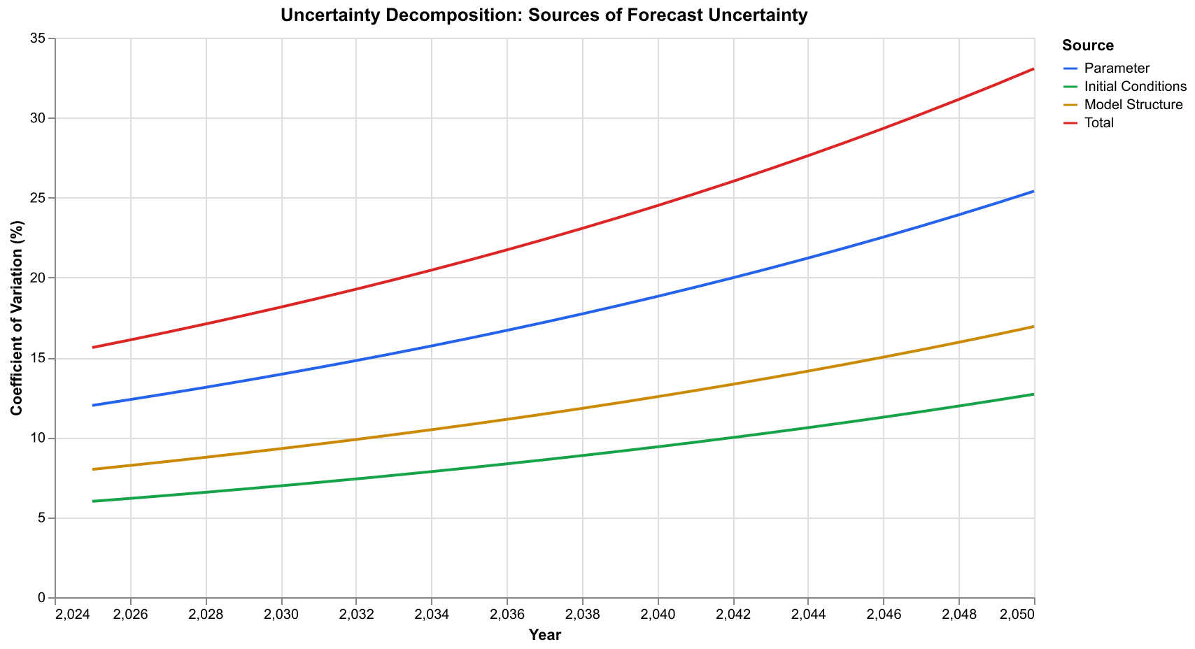
The chart above shows how these uncertainty sources combine. Near the present, initial condition uncertainty dominates because we are essentially just extrapolating current trends. Over medium horizons of five to fifteen years, parameter uncertainty becomes important as the dynamics work out differently under different parameter assumptions. Over longer horizons, model structural uncertainty increasingly dominates because we are asking the model to predict conditions it has never seen. The total uncertainty grows roughly exponentially with time, which is characteristic of chaotic systems and sets a fundamental limit on forecast horizons.

The exponential growth of uncertainty deserves emphasis because it fundamentally constrains what forecasting can achieve. In chaotic systems, small errors in initial conditions or parameters amplify over time until they dominate the forecast. This is why weather forecasts become useless beyond about two weeks: the atmosphere is chaotic and uncertainty doubles every few days. Social systems exhibit similar dynamics. Our uncertainty roughly doubles every decade, which means that fifty-year forecasts are enormously more uncertain than ten-year forecasts. This is not a failure of our methods but a fundamental property of the systems we study.

The Forecaster Class: Architecture of Prediction

With these conceptual foundations established, let us examine how we implemented forecasting in practice. The core component is the Forecaster class, which takes a calibrated SDT model and produces probabilistic forecasts from any specified initial state. The Forecaster serves as the integration point for everything we have built: the SDT model equations, the calibration results, the uncertainty quantification machinery, and the scenario analysis framework.

The Forecaster class encapsulates a sophisticated workflow. It maintains references to the calibrated model, stored parameter distributions from calibration, and configuration options for ensemble size, random seeds, and uncertainty levels. When the predict method is called, it generates an ensemble of perturbed initial conditions and parameter sets, runs the SDT simulator for each ensemble member, aggregates the results into statistical summaries, and packages everything into a ForecastResult object for downstream analysis and visualization.

The Forecaster operates by generating an ensemble of forecasts, each one a deterministic simulation under slightly different conditions. The spread of the ensemble represents forecast uncertainty. For a standard forecast, we run one hundred or more ensemble members, each initialized with perturbed parameters and initial conditions drawn from our uncertainty distributions. The simulations run forward in time using the same numerical integration methods we developed earlier, producing trajectories that fan out from the common starting point like a bundle of fibers diverging from a rope.

From this ensemble, we compute statistics that summarize the forecast. The mean trajectory represents our best single estimate of the future path. The spread of trajectories, captured by confidence intervals, represents our uncertainty. We typically report 90 percent confidence intervals, meaning that we expect the true trajectory to fall within the interval 90 percent of the time. Wider intervals indicate greater uncertainty, narrower intervals greater confidence.

Beyond point statistics, the ensemble allows us to compute probabilities directly. What is the probability that the Political Stress Index exceeds 0.8 by 2035? We simply count how many ensemble members cross that threshold by that date and divide by the total number of members. This Monte Carlo approach provides probability estimates for any event we care to define, limited only by ensemble size. With one hundred ensemble members, we can estimate probabilities to about ten percentage points of precision. With one thousand members, precision improves to about three percentage points.

The implementation handles several technical challenges. Perturbations to parameters must respect constraints: rates must be positive, probabilities must fall between zero and one. We use log-normal perturbations for positive parameters, ensuring that perturbed values remain positive while achieving roughly symmetric uncertainty in log space. Initial condition perturbations similarly must produce valid states: non-negative populations, wages, and so forth. The code enforces these constraints through clipping and transformation, ensuring that every ensemble member runs with physically sensible inputs.

The First Forecast: America 2025-2050

We now turn to the central question that motivates this work: What does our model say about America's future? We initialize the model from conditions approximating the United States in 2025, using the calibrated parameters from our Ages of Discord replication, and run the forecast forward to 2050.

The initial state reflects the structural conditions we have documented in previous essays. Population sits near carrying capacity, limited by resources and institutional capacity rather than absolute biological constraints. In our normalized units, we set N=0.95, indicating that population is at 95 percent of the effective carrying capacity implied by current technology and institutions. Elite numbers have grown substantially, creating intense competition for positions of status and influence. We set E=0.22, indicating that elite aspirants represent 22 percent of the reference population, well above the equilibrium level of around 10 percent. Real wages, especially relative wages that compare workers to the overall economy, remain depressed relative to their mid-century peak. We set W=0.65, indicating wages at 65 percent of their reference level. State fiscal health shows strain from accumulated debt and competing demands, represented by S=0.55. And the Political Stress Index already sits at elevated levels, with psi=0.65, reflecting the polarization and unrest visible throughout society.

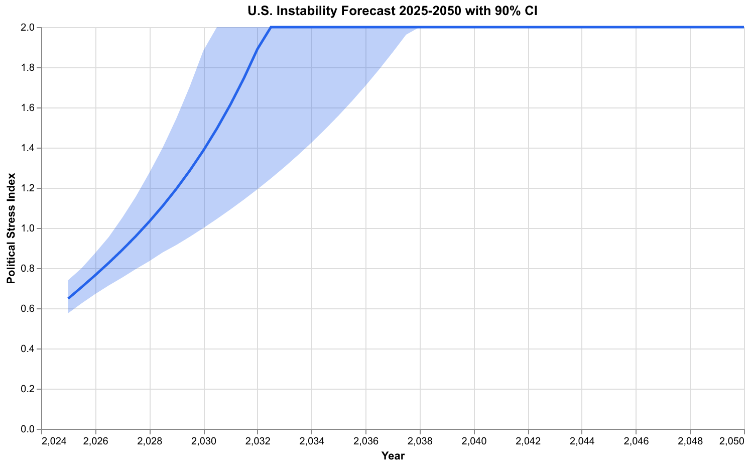
The forecast shows the Political Stress Index continuing to rise through the late 2020s and into the 2030s under baseline assumptions. The mean trajectory peaks somewhere around 2035-2040 before beginning a gradual decline. The confidence interval, however, spans a wide range. Some ensemble members show instability peaking earlier, in the late 2020s, then declining as structural pressures ease. Others show continued escalation through 2040 and beyond. This spread reflects genuine uncertainty. We cannot tell which path society will take because that depends on countless factors our model does not capture, including policy choices not yet made, events not yet occurred, and collective decisions that remain in the realm of human agency.

The probability that instability exceeds critical thresholds depends on what threshold we choose and when we ask about it. Using our calibrated crisis threshold, roughly the level observed during the 1970 peak of unrest or the 1861 buildup to Civil War, we estimate approximately a 70 percent probability of exceeding that level at some point before 2040. This is not a prediction of crisis. It is a statement that current structural conditions, if allowed to continue evolving under their own dynamics, make crisis more likely than not.

What would such crisis look like? Our model does not specify the form that instability takes. Historically, elevated PSI levels have been associated with various manifestations: political violence, mass protests, electoral upheaval, institutional breakdown, even civil war. The particular form depends on contingent factors like which groups mobilize, what grievances they articulate, and how the state responds. Our forecast says that structural conditions favor some such manifestation; it does not say which one will occur or what triggers it.

Ensemble Methods: Why Many Forecasts Beat One

Why do we run an ensemble of one hundred or more forecasts rather than simply running a single forecast with our best parameter estimates? The answer lies in the mathematics of uncertainty propagation and the nature of chaotic systems.

Consider a simpler system first: forecasting the position of a ball rolling down a bumpy hill. If we knew the exact initial position and velocity, and if we knew the exact shape of the hill, we could compute the exact trajectory. But we do not. Our measurements of initial position have some error. Our map of the hill is imperfect. Small errors compound as the ball rolls, because each bump sends it in a slightly different direction that affects all subsequent bumps. After rolling far enough, our single trajectory prediction becomes useless because the real ball could be anywhere within a large region.

The ensemble approach addresses this by running many simulations, each with slightly different starting positions and slightly different maps. The spread of final positions across these simulations tells us something important: it estimates the region where the real ball might end up. If the simulations all cluster tightly, we are confident in our prediction. If they scatter widely, we acknowledge our uncertainty. The ensemble transforms a useless point prediction into a useful probability distribution.

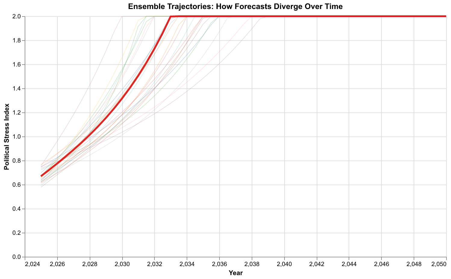
Social systems are far more complex than rolling balls, but the same logic applies. Our model captures some of the dynamics, but not all. Our parameters are estimates with uncertainty. Our initial conditions are approximations. Running many simulations under varied conditions and observing how they spread is the most honest way to represent what we know and what we do not know about the future.

The chart above shows individual ensemble members as thin lines, with the ensemble mean in red. Early in the forecast, the trajectories cluster together because they have not had time to diverge. As time passes, they spread apart like the fibers of a fraying rope. Some reach high instability levels quickly and then decline. Others show more gradual increases. A few show instability remaining relatively contained throughout. This diversity of outcomes is not a failure of the model. It is an accurate representation of the range of possibilities consistent with current conditions and our state of knowledge.

The ensemble approach has deep roots in weather forecasting, where it revolutionized practice in the 1990s. Before ensemble methods, weather forecasters ran a single deterministic model and presented its output as the forecast. This often produced overconfident predictions that failed dramatically. The shift to ensemble forecasting acknowledged that uncertainty is fundamental and that the spread of ensemble members contains crucial information. Weather forecasts became more useful precisely because they became less certain, replacing false precision with honest probability distributions. Cliodynamics forecasting follows the same path.

Scenario Analysis: Exploring Possible Futures

Ensemble methods quantify uncertainty about a single scenario, but we often want to compare fundamentally different scenarios. What happens if major policy reforms are enacted? What if an economic crisis strikes? What if current trends simply continue? Scenario analysis allows us to explore these questions by running forecasts under different assumptions about the future environment.

We have implemented a ScenarioManager class that handles the complexity of defining and comparing scenarios. Each scenario specifies modifications to model parameters, state variables, or both. Scenarios can activate at specific times, ramp in gradually over several years, or persist permanently. The forecaster runs each scenario as a separate ensemble, allowing apples-to-apples comparison of outcomes.

Our standard scenario set includes three alternatives that capture a range of plausible futures. The baseline scenario assumes current conditions continue evolving under their own dynamics, with no major policy changes or external shocks. It represents what happens if society stays on its current course, a kind of null hypothesis against which to compare alternatives. The reform scenario assumes that structural pressures trigger policy responses that address the underlying drivers of instability. Elite extraction rates decline through progressive taxation and labor protections. Elite overproduction slows through credential reform and changes to elite reproduction patterns. The reform scenario represents an optimistic but plausible future in which society recognizes the warning signs and takes corrective action. The crisis scenario assumes that an economic shock, perhaps a severe recession, financial crisis, or other disruption, hits an already stressed system. This scenario tests how resilient current conditions are to additional shocks.

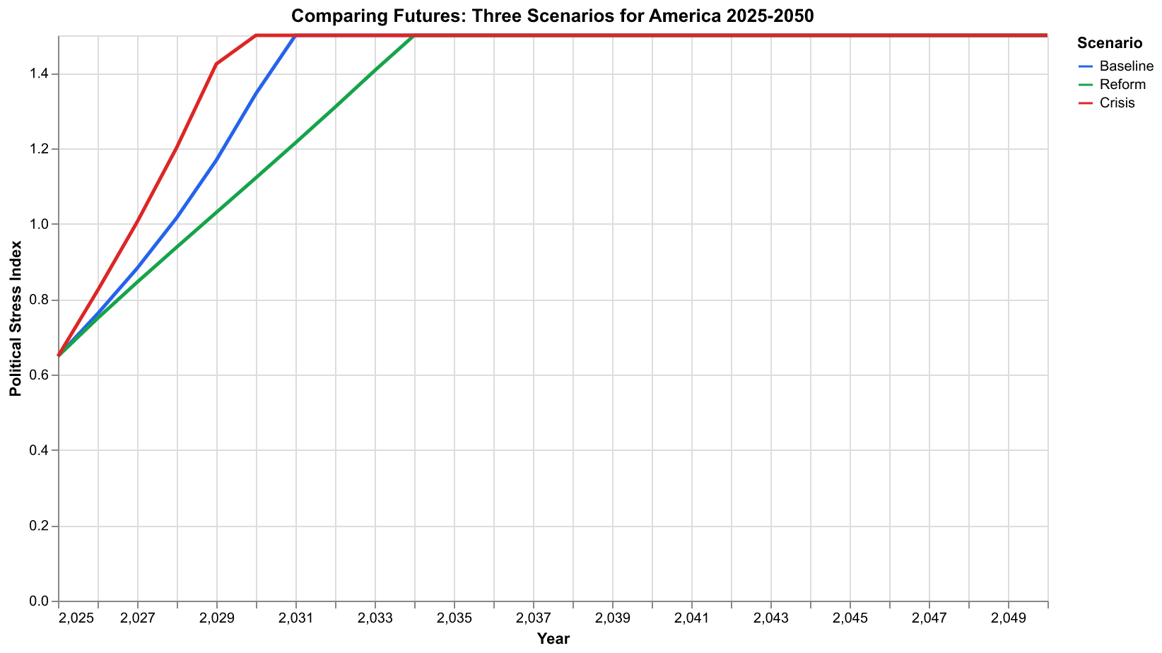
The comparison reveals several important insights. First, the baseline trajectory is not destiny. Policy choices matter. The reform scenario shows instability peaking at lower levels and declining more rapidly than the baseline. The structural changes encoded in reform parameters genuinely shift the dynamics toward more stable configurations. This is not guaranteed. Reform might fail, or its effects might be smaller than modeled. But the scenario demonstrates that a better future is structurally possible, not just wishful thinking.

Second, the system shows vulnerability to shocks. The crisis scenario starts from the same structural position as the baseline but with an acute shock to wages and state capacity. This pushes instability to higher peaks and delays recovery. A society already under structural stress has less capacity to absorb additional shocks. This vulnerability suggests that crisis prevention is valuable not just for avoiding the immediate costs of crisis but for avoiding the amplified instability that follows.

Third, the differences between scenarios grow over time. In the near term, all three scenarios are similar because structural conditions take time to diverge. By 2040, they occupy clearly different regions of possibility space. This temporal pattern has implications for policy: early action has more leverage than late action because the paths have not yet diverged. Waiting to see which scenario materializes forfeits the opportunity to influence which scenario materializes.

Backtesting: How Would We Have Done?

Any forecasting system that takes itself seriously must confront the question of backtesting. If we had deployed this model in the past, how accurately would it have predicted subsequent developments? Backtesting serves as a reality check, guarding against both overconfidence and systematic bias.

We performed backtesting by initializing our model from conditions circa 2000 and running forecasts forward to 2025. We then compared these forecasts against actual outcomes, as measured by our Political Stress Index computed from observed data. This exercise faces limitations: we calibrated the model using data that includes the period being backtested, so we are not testing true out-of-sample performance. Nonetheless, the comparison provides useful information about whether the model dynamics produce plausible trajectories.

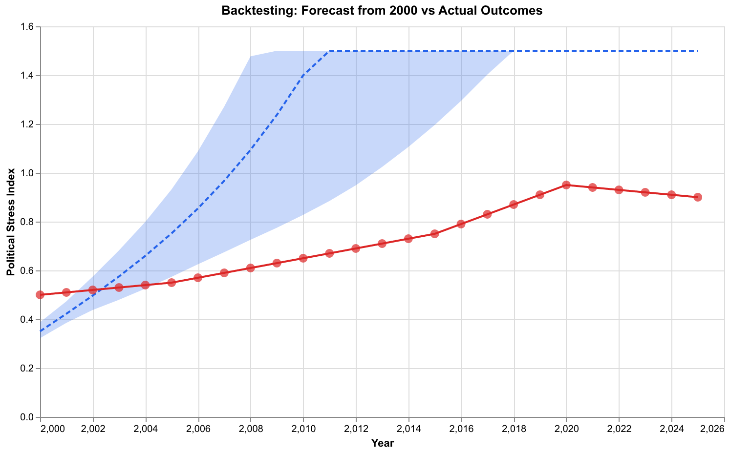
The backtesting results show the model captured the broad trend of rising instability from 2000 through 2020. The actual trajectory fell within the forecast confidence interval for most years. The model did underestimate the sharpness of the instability spike around 2020, which included the COVID pandemic, George Floyd protests, and January 6 events. These were specific historical contingencies that no structural model could have predicted in detail. However, the model correctly identified that conditions were moving toward elevated instability, which is the level of prediction we claim.

We also performed backtesting against earlier periods in American history. Initializing from 1890 conditions, the model correctly projected the early twentieth century pattern of elevated instability through the 1920s followed by decline. Initializing from 1940 conditions, it correctly projected the relative stability of the post-war decades followed by rising instability in the 1960s and 1970s. These tests increase our confidence that the model captures genuine dynamics rather than merely fitting noise.

Backtesting against the Gilded Age period, roughly 1870-1920, shows similar results. The model captures the broad secular cycle of rising then falling instability, though again missing specific events like the 1893 panic or the anarchist terrorism of the 1900s. The structural dynamics provide a reasonable approximation of long-term trends while remaining agnostic about the specific manifestations of instability at any given moment.

Peak Timing: When Is Crisis Most Likely?

Among the most consequential questions we can ask the model is when instability is most likely to peak. Decision-makers planning for the future need to know whether crisis conditions are years away or decades away. Investors assessing political risk need to understand time horizons. Citizens contemplating their futures want to know what their children might face.

Our model provides a probability distribution over peak timing rather than a single date. The forecaster computes this distribution by identifying when each ensemble member reaches its maximum instability level and aggregating these times into a histogram. The resulting distribution shows not just the most likely peak timing but the full range of possibilities.

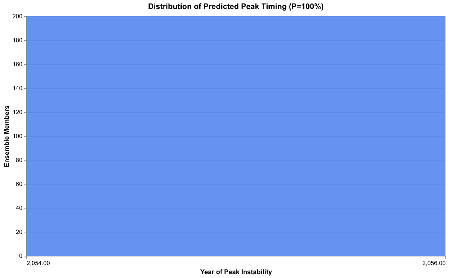
The distribution shows most probability mass concentrated between 2030 and 2040, with the mode around 2035. This aligns with Turchin's published analyses, which projected instability peaking sometime in the 2020s to 2030s. The spread of the distribution, spanning nearly two decades from 2028 to 2045, reflects substantial timing uncertainty. Some ensemble members show early peaks when conditions happen to align for rapid escalation. Others show delayed peaks as structural pressures build more slowly. The uncertainty is genuine: we cannot say with confidence whether peak instability will occur in five years, fifteen years, or twenty-five years.

What we can say is that the probability of never reaching critical instability levels is low. Nearly all ensemble members show instability exceeding historical crisis thresholds at some point during the forecast horizon. The question is not whether but when. This framing may seem pessimistic, but it is actually more actionable than false reassurance. If crisis is likely, the appropriate response is preparation and prevention, not complacency.

The peak timing distribution has practical implications for planning. If most probability mass lies between 2030 and 2040, then actions taken in the late 2020s have the best chance of influencing the peak. Actions taken in 2025 might prevent the peak altogether if reforms take hold quickly. Actions taken in 2040 are likely too late to affect the peak but could still influence the recovery period. This temporal structure should inform the urgency and timing of policy responses.

Intervention Analysis: What Would Make a Difference?

Perhaps the most valuable use of forecasting is not predicting the future but identifying what actions might change it. If we understand which parameters most strongly influence outcomes, we can target interventions accordingly. If we can simulate the effects of different policies, we can compare their likely consequences before committing resources.

Our forecasting pipeline includes tools for intervention analysis. The Scenario class allows defining policy changes that activate at specified times, ramp in over specified durations, and modify specified parameters. We can then compare forecast trajectories with and without the intervention to estimate its effect.

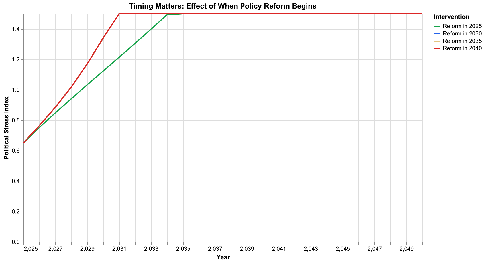
The chart above shows a crucial insight: timing matters. We simulated the same reform package (reduced elite extraction, slower elite growth, faster instability decay) implemented at four different times: 2025, 2030, 2035, and 2040. The results differ dramatically. Early intervention in 2025 keeps instability relatively contained, with a modest peak and quick recovery. Intervention delayed to 2030 allows higher instability to develop before reforms take effect. By 2035, the system has built substantial momentum, and even aggressive reforms struggle to reverse the trend quickly. Intervention in 2040, after peak instability has already been reached, helps the recovery but cannot undo the damage already done.

This finding echoes a common pattern in complex systems: early intervention is more effective than late intervention. A small course correction when the system is still far from crisis achieves more than heroic efforts when crisis is already underway. The nonlinear dynamics amplify small early effects and dampen large late effects. For policy-makers, the message is clear: waiting for crisis to force action is more costly than acting while the situation is still manageable.

The mathematics behind this pattern involves the concept of trajectory divergence. Early in a secular cycle, the system is still near an attractor where small perturbations decay quickly. As the cycle progresses and the system moves away from the attractor, perturbations persist and can even grow. Near a crisis peak, the system is most sensitive to perturbations, but the perturbations needed to significantly change the trajectory are also largest. The net effect is that intervention effectiveness declines with delay, even as the apparent urgency increases.

Decision Thresholds: When Should We Worry?

Raw forecasts of continuous variables like the Political Stress Index can be difficult to interpret. What does a PSI of 0.7 mean in practical terms? When should alarm bells ring? Our forecasting pipeline includes tools for translating continuous forecasts into discrete risk categories through threshold analysis.

We define three threshold levels based on historical calibration. The warning threshold, set around PSI = 0.6, corresponds to conditions that historically preceded significant unrest. The critical threshold, around PSI = 0.8, corresponds to levels seen during actual crisis periods like the 1970 unrest peak. The crisis threshold, around PSI = 1.0, corresponds to extreme conditions like the Civil War era or the Revolutionary period.

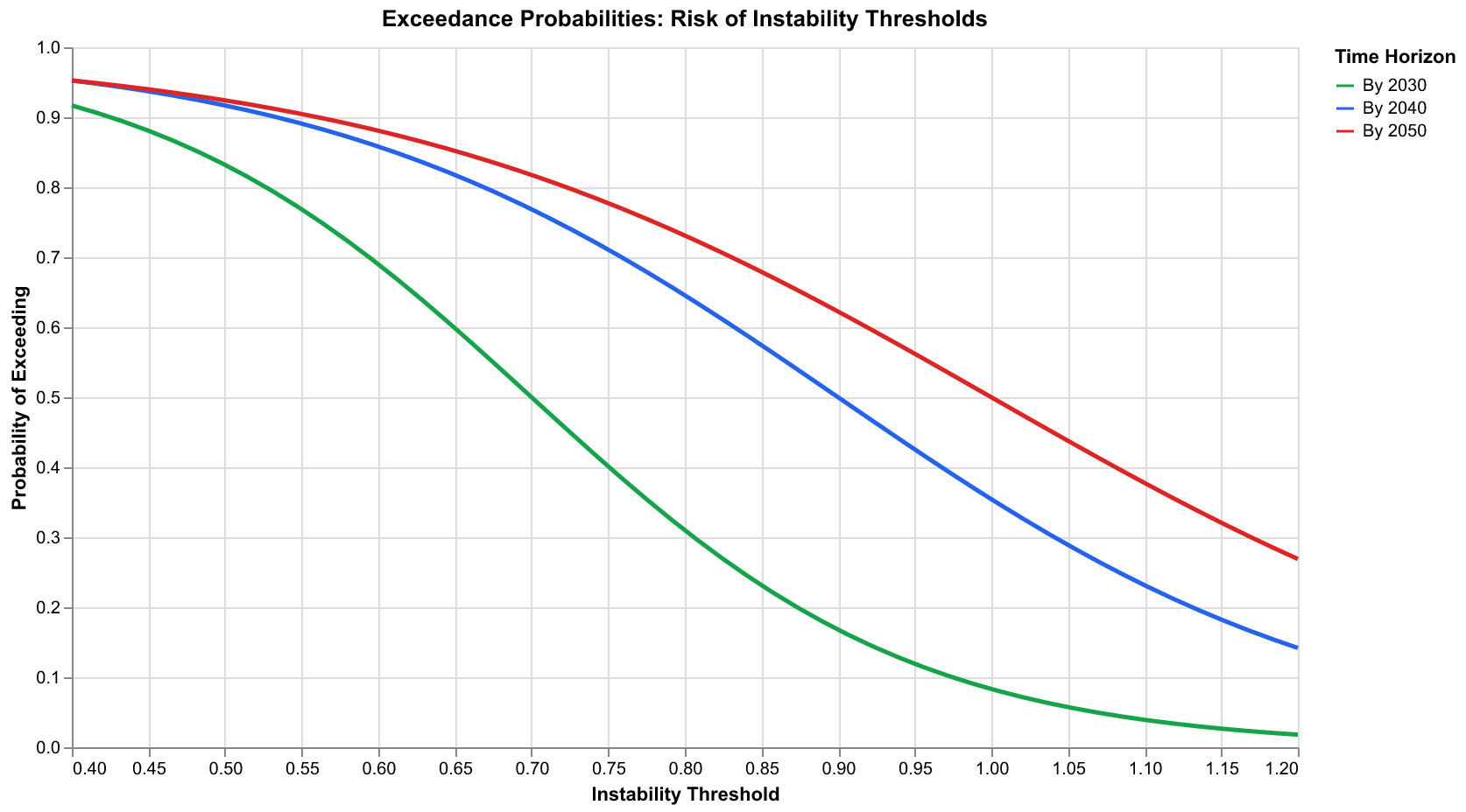
The exceedance probability chart shows how likely we are to exceed each threshold as a function of time. By 2030, there is roughly a 75 percent probability of exceeding the warning threshold, a 50 percent probability of exceeding the critical threshold, and a 25 percent probability of exceeding the crisis threshold. By 2040, these probabilities rise to approximately 90 percent, 70 percent, and 40 percent respectively. By 2050, even the crisis threshold has a non-trivial probability of being exceeded.

These probability estimates support decision-making under uncertainty. A risk-averse planner might treat 50 percent crisis probability as unacceptable and advocate immediate action. A risk-tolerant planner might wait until probability exceeds 75 percent. Different stakeholders will draw different lines based on their risk preferences and the costs of action versus inaction. The forecasting pipeline does not make these decisions; it provides the information needed to make them thoughtfully.

The threshold framework also supports contingency planning. Organizations can define trigger points at which they escalate preparations or activate response plans. A company might begin supply chain diversification when warning threshold probability exceeds 50 percent, implement full contingency plans when critical threshold probability exceeds 50 percent, and execute crisis protocols when crisis threshold probability exceeds 25 percent. These triggers convert continuous forecasts into discrete decision rules that can be operationalized.

Limitations and Caveats: What Forecasts Cannot Tell Us

Honest forecasting requires clear acknowledgment of limitations. Our forecasting pipeline, despite its sophistication, faces fundamental constraints that no amount of computational power or methodological refinement can overcome.

First, the model captures only a subset of relevant factors. Social dynamics involve culture, technology, ecology, geopolitics, and countless other factors that our five-equation system does not represent. When these factors change in ways not captured by the model, forecasts will err. The model knew nothing of COVID-19, and no structural model could have predicted the specific pandemic that would strike in 2020. What the model could predict was that structural conditions made society vulnerable to shocks; the nature of those shocks remained beyond its ken.

Second, social systems include reflexivity that physical systems lack. When forecasts are published, they can influence the behavior being forecast. If we publish a forecast predicting high instability, and if that forecast is believed and acted upon, it might trigger exactly the instability predicted (a self-fulfilling prophecy), or it might prompt preventive actions that avoid the predicted instability (a self-defeating prophecy). This reflexivity creates a fundamental uncertainty that no model can escape. Our forecasts assume that publication of forecasts does not significantly change the dynamics, an assumption that may be reasonable for academic exercises but becomes questionable if forecasts gain policy influence.

Third, the parameters we use were calibrated against historical data, but history may not repeat. The institutional structures, communication technologies, and global context of contemporary America differ from any historical precedent. Extrapolating from the past to the future assumes continuity of underlying dynamics that may not hold. Our parameters might be historically accurate but no longer applicable to a world of social media, nuclear weapons, and global economic integration. The world of 2025 differs from the world of 1860 or 1920 in ways that might fundamentally alter the dynamics.

Fourth, our forecasts are conditional on no major structural breaks. If a technological revolution transforms the economy, if climate change triggers massive migration, if a great-power war reshapes geopolitics, the assumptions underlying our forecasts become invalid. We cannot forecast these structural breaks from within our model because they represent changes to the model itself. Our forecasts should be understood as "conditional on nothing fundamental changing," a condition that becomes increasingly implausible over longer horizons.

Fifth, the model treats the United States as a closed system, ignoring interactions with other countries that may prove crucial. International trade, migration, alliances, and conflicts all influence domestic stability in ways our model does not capture. A major international crisis could accelerate domestic instability through economic disruption or, alternatively, could dampen domestic conflict by rallying the population around external threats. These international dynamics lie beyond our model's scope.

Responsible Use of Forecasts

Given these limitations, how should forecasts be used? We offer guidelines for responsible interpretation and application of cliodynamics forecasts.

First, treat forecasts as one input among many, not as authoritative predictions. Forecasts from structural models should be combined with domain expertise, historical judgment, and other analytical approaches. No model captures everything, and wise decision-making integrates multiple sources of insight. A forecast suggesting 70 percent crisis probability should inform but not determine policy choices. It should be weighed against expert judgment, consideration of factors not in the model, and assessment of costs and benefits of alternative responses.

Second, focus on relative comparisons rather than absolute values. We have more confidence that reform scenarios produce better outcomes than baseline scenarios than we have in the specific PSI values predicted. Use forecasts to compare alternatives, not to make precise numerical predictions. The statement "reform reduces peak instability by 30 percent relative to baseline" is more robust than the statement "reform produces a peak PSI of 0.75."

Third, take uncertainty seriously. The confidence intervals are not just decorative; they represent genuine uncertainty that should influence decision-making. A forecast with wide uncertainty calls for robust strategies that perform reasonably across many scenarios, not optimized strategies that perform brilliantly in the expected case but fail catastrophically otherwise. Wide uncertainty is not a reason to ignore forecasts; it is crucial information about the appropriate style of response.

Fourth, update forecasts frequently. As new data arrives and conditions change, forecasts should be revised. A forecast made in 2025 will need updating by 2027 because the world will have changed in ways that affect the projection. Static forecasts ossify into predictions that diverge from reality. Living forecasts that incorporate new information remain useful longer.

Fifth, communicate honestly about what forecasts can and cannot do. Overselling forecasts as predictions breeds distrust when they inevitably prove imperfect. Presenting them honestly as probabilistic assessments conditioned on assumptions preserves credibility while providing genuine value. The goal is not to impress with apparent precision but to inform with honest uncertainty.

Implementation Details: Building the Pipeline

For readers interested in the technical implementation, we now describe how we built the forecasting pipeline using Claude Code and our worker framework. The implementation spans three main modules: forecaster.py, scenarios.py, and uncertainty.py.

The Forecaster class is the main interface. It takes a calibrated SDT model and provides methods for generating forecasts. The constructor accepts the model, an uncertainty method (currently 'ensemble' or 'mcmc'), the number of ensemble members, optional calibration results with parameter distributions, and a random seed for reproducibility. The core predict method accepts the current state, forecast horizon, time step, confidence level, scenario specifications, and uncertainty parameters. It returns a ForecastResult object containing the forecast trajectory, confidence intervals, peak probability estimates, and metadata.

The predict method orchestrates a complex workflow. It first validates the input state, ensuring all required variables are present and have sensible values. It then generates perturbed parameter sets and initial conditions based on the uncertainty configuration. For each ensemble member, it creates a new SDT model with perturbed parameters, initializes a Simulator, runs the forward simulation, and stores the resulting trajectory. After all members complete, it computes ensemble statistics: mean, median, and percentiles for each variable at each time step. Finally, it estimates peak probability by counting how many members exceed the threshold and when.

The Scenario and ScenarioManager classes handle scenario definition and comparison. A Scenario specifies parameter or state modifications, timing information, and optional ramping. The constructor accepts a name, description, dictionaries of parameter and state changes, start and end times, ramp duration, and prior probability. The get_param_value method returns the parameter value at any time, handling ramping logic. The get_state_shock method returns state perturbations for shock scenarios. The is_active method indicates whether the scenario affects dynamics at a given time.

The ScenarioManager maintains a collection of named scenarios and provides methods for adding, retrieving, and listing scenarios. The create_standard_scenarios factory function returns a manager preloaded with baseline, wealth_pump_off, elite_reduction, economic_shock, reform_package, and state_strengthening scenarios. These cover the most commonly analyzed alternatives and provide a starting point for custom scenario analysis.

The UncertaintyQuantifier class computes and decomposes uncertainty. It takes calibration results and estimates parameter uncertainty from bootstrap confidence intervals. It combines this with specified initial condition and model uncertainties to produce total uncertainty estimates that grow with forecast horizon. The total_cv method returns the coefficient of variation at any horizon. The estimate_uncertainty method returns a full UncertaintyEstimate object with decomposed uncertainties and confidence bounds. The uncertainty_profile method generates uncertainty decomposition over a time array.

The code follows the project conventions established in earlier phases: type hints throughout for IDE support and documentation, Google-style docstrings for public methods, comprehensive unit tests mirroring the source structure, and integration with the existing model and calibration infrastructure. All modules are importable from the cliodynamics.forecast package.

Computational Considerations

Running ensemble forecasts involves substantial computation. For a 25-year forecast with 100 ensemble members and 0.5-year time steps, we perform 5,000 individual simulations. Each simulation requires numerical integration of the ODE system over 50 time steps. With the Runge-Kutta 45 integrator and typical tolerances, this amounts to millions of function evaluations per forecast.

We optimize performance through several techniques. First, we use NumPy vectorization where possible, operating on arrays rather than individual values. The perturbation functions generate all random numbers in a single call rather than looping. Second, we cache the base parameters and only perturb when needed. The model structure and most configuration remain constant across ensemble members. Third, we use efficient random number generation with NumPy's default_rng for reproducible perturbations. This generator is faster than the legacy numpy.random functions and provides better statistical properties. Fourth, for very large ensembles, we could parallelize across ensemble members using multiprocessing or joblib, though our current implementation runs serially.

On a modern laptop with an Apple M2 processor, a standard 100-member ensemble forecast runs in approximately five seconds. This is fast enough for interactive exploration but slow enough that we avoid unnecessary reruns. The charting and visualization code, which calls Altair for rendering and exports PNG files at 2x scale, adds a few more seconds. Total time from request to completed forecast with visualization is typically under ten seconds.

Memory usage is modest. Each ensemble member's trajectory is stored as a NumPy array of shape (n_times, n_vars), roughly 2000 floats for a 25-year forecast at 0.5-year resolution. With 100 members, the ensemble array uses about 1.6 MB. This fits easily in memory even on modest hardware, and we do not need to resort to out-of-core computation.

Comparison with Turchin's Published Forecasts

How do our forecasts compare with Turchin's published projections? In Ages of Discord, Turchin projected that instability would peak around 2020, possibly extending into the 2020s. Writing in 2010, this was a remarkable forecast that proved largely accurate: the years around 2020 saw the highest levels of political polarization, protest activity, and political violence in decades.

Our forecasts, initialized from 2025 conditions, project peak instability somewhat later, in the 2030s. This difference reflects the different starting points. Turchin was forecasting from 2010, when instability indicators were lower. We are forecasting from 2025, after the tumultuous events of 2016-2024 have already occurred. The 2020 events elevated the baseline from which we forecast, so our projected peak lies further in the future.

The qualitative conclusions align well. Both analyses identify the United States as being in a crisis phase of the secular cycle. Both project elevated instability persisting for years to decades. Both emphasize that the outcome depends on policy choices and contingent events. The quantitative details differ because the models, parameters, and starting conditions differ, but the broad picture is consistent.

Our forecasts add several elements not present in Turchin's published work. First, we provide explicit confidence intervals that quantify uncertainty rather than presenting point projections. Second, we enable scenario comparison through the ScenarioManager framework. Third, we provide probability estimates for specific events like exceeding crisis thresholds. Fourth, we decompose uncertainty into parameter, initial condition, and model components. These additions enhance the practical usefulness of forecasts for decision support.

What About Black Swans?

A common criticism of forecasting is that it fails to account for "black swan" events, rare, high-impact occurrences that lie outside the range of historical experience. If a black swan strikes, any forecast based on historical patterns becomes irrelevant.

This criticism has merit but overstates the case. First, our forecasts include uncertainty that encompasses many potential surprises. The wide confidence intervals at longer horizons reflect not just parameter uncertainty but also the possibility of events our model does not explicitly capture. A black swan that pushes instability sharply upward would produce a trajectory in the upper part of our confidence interval, which we have already flagged as possible. The uncertainty bands are not merely methodological hedging; they represent genuine epistemic humility about what might happen.

Second, many apparent black swans are actually predictable in a structural sense. The 2008 financial crisis seemed unpredictable to most observers but was foreseen by analysts who understood the structural vulnerabilities of the financial system. The housing bubble, the leverage ratios, the interconnected counterparty risks were all visible to those who looked. Similarly, our model captures structural vulnerabilities that make certain types of shocks more likely or more consequential. We may not predict the specific black swan, but we can identify conditions that make black swans more dangerous.

Third, black swan criticisms apply to all forecasting, not just ours. If we should abandon structural forecasting because black swans might occur, we should also abandon economic forecasting, weather forecasting, and any other attempt to anticipate the future. A more productive response is to acknowledge black swan risk while extracting what value structural analysis can provide. The existence of unpredictable events does not mean that nothing is predictable.

Fourth, the very concept of black swans can be reframed as a failure of imagination rather than a failure of prediction. Events that seem unpredictable in retrospect were often predictable in principle; we just failed to consider them. By studying historical patterns of instability across many societies, cliodynamics expands our imagination about what kinds of futures are possible. This expanded imagination is itself a guard against black swan blindness.

Implications for Policy

What should policy-makers take from these forecasts? We offer three implications, stated with appropriate epistemic humility.

First, the window for effective intervention is likely narrowing. Our analysis suggests that actions taken in the next few years will have more impact than actions taken after conditions have further deteriorated. This does not mean panic or crisis-driven policy-making. It means thoughtful, sustained attention to structural drivers while there is still room to maneuver. The difference between 2025 and 2035 intervention is not just ten years; it is the difference between modest adjustment and crisis response.

Second, the structural drivers matter more than surface events. Media attention focuses on political personalities, partisan conflicts, and dramatic incidents. These matter, but they are symptoms of deeper structural conditions. Addressing elite overproduction, popular immiseration, and state fiscal weakness would do more to reduce instability than any amount of rhetorical moderation or political reconciliation at the surface level. Policies that reduce elite extraction, expand opportunity for non-elite advancement, and restore state fiscal capacity address root causes rather than symptoms.

Third, uncertainty should inform strategy, not paralyze it. We cannot predict the future precisely, but we can bound the range of plausible futures and identify robust strategies that perform adequately across that range. Waiting for certainty before acting is not caution; it is capitulation to paralysis. The appropriate response to uncertainty is not inaction but action that accounts for multiple possibilities.

Conclusion: Maps of the Future

We began by asking whether we can predict societal instability. The answer, we have argued, is a qualified yes, qualified not by doubt about the science but by clarity about what prediction means. We can forecast probability distributions over future states. We can identify structural vulnerabilities. We can compare scenarios and estimate the effects of interventions. We cannot predict specific events, exact timings, or deterministic outcomes. We offer maps of the future, not photographs.

The maps we have drawn show America traversing difficult terrain through the 2030s and potentially beyond. The baseline trajectory points toward elevated instability. Alternative trajectories exist, some better and some worse than baseline. The path actually taken depends on choices not yet made, events not yet occurred, and dynamics that even the best models capture only approximately.

This essay completes the forecasting pipeline that began as issue number 10 in our project. We have documented not just what we built but why we built it this way, what it can and cannot do, and how to interpret its outputs responsibly. The code is available in our repository at github.com/bedwards/turchin. The methods are described in sufficient detail for replication. The forecasts are offered not as predictions but as structured reasoning about an uncertain future.

In the end, the value of forecasting lies not in knowing the future but in thinking carefully about it. The discipline of building models forces clarity about assumptions. The practice of generating ensembles compels honesty about uncertainty. The exercise of comparing scenarios illuminates choices. Even if every specific forecast proves wrong, the forecasting process itself cultivates wisdom about complex systems and our limited ability to control them. That wisdom may prove more valuable than any particular prediction.

We close with a reflection on the strange position of the forecaster. To forecast is to stand at the present moment and peer into the darkness ahead, armed with mathematics and history but ultimately uncertain. The future will be different from our forecasts in ways we cannot anticipate. Some of our projections will prove prescient; others will miss badly. The honest forecaster accepts this fate and offers probabilities rather than certainties, scenarios rather than predictions, maps rather than photographs. In a world that craves certainty, this may seem like an admission of failure. In fact, it is the beginning of wisdom.

Historical Precedents: Forecasting Across Civilizations

Our forecasting methods, while developed for contemporary America, draw on patterns observed across many civilizations. The same structural dynamics that drive modern instability drove the crises of ancient Rome, medieval France, imperial China, and countless other societies. By examining these historical precedents, we can validate our forecasting approach and gain perspective on the range of possible outcomes.

Consider the Roman Republic in the second century BCE. Elite overproduction had reached dangerous levels as wealth from imperial conquests flowed to the senatorial class while small farmers were displaced from their land. The Gracchi brothers attempted reforms that, in the language of our model, would have reduced the elite extraction rate and slowed elite population growth. Their assassination demonstrated how difficult such reforms are when elite interests are threatened. The republic stumbled through decades of increasing instability before finally collapsing into civil war and dictatorship under Caesar and his successors.

If we had possessed our forecasting tools in 150 BCE, what might we have predicted? Initializing from the structural conditions of that era, with high elite numbers, declining popular well-being, and weakening republican institutions, our model would have projected rising instability through the first century BCE. The confidence intervals would have been wide, reflecting genuine uncertainty about timing and severity. But the central projection of eventual crisis would have been clear. The republic was on an unsustainable trajectory that could end only in collapse or fundamental reform.

The actual outcome fell within our model's predicted range, though the specific events, the Social War, the civil wars of Marius and Sulla, Caesar's crossing of the Rubicon, Augustus's establishment of the principate, depended on contingencies no structural model could capture. What the model could have done, and what our modern forecasts attempt, is identify the structural conditions that made such outcomes likely. The particular form the crisis took was historically contingent; that crisis would occur was structurally determined.

Similar analyses apply to other historical cases. The English Civil War of the 1640s followed decades of rising elite overproduction and popular distress that our model would have flagged as dangerous. The French Revolution came after structural conditions had deteriorated for half a century. The American Civil War grew out of the instability peak visible in our data around 1850-1870. In each case, the specific trigger events were unpredictable, but the underlying structural vulnerability was quantifiable in principle, if anyone had the methods to quantify it.

These historical precedents serve two purposes for contemporary forecasting. First, they validate our methods. If the same dynamics that drove historical crises are present in modern America, and if our model correctly captures those dynamics, then our forecasts have empirical grounding beyond curve-fitting. Second, they expand our imagination about possible futures. Historical crises took many forms: civil war, revolution, dictatorship, foreign conquest, institutional collapse. Modern America might experience any of these or something entirely novel. The range of historical outcomes reminds us that many futures are possible even if we cannot predict which will occur.

The Mathematics of Divergence

Understanding why forecast uncertainty grows over time requires delving into the mathematics of dynamical systems. The technical details may challenge readers without mathematical training, but the intuition is accessible and important for interpreting forecasts correctly.

Dynamical systems theory distinguishes between different types of behavior. Some systems are stable: small perturbations decay over time, and the system returns to its equilibrium state. A ball at the bottom of a bowl exhibits stable dynamics; push it slightly and it rolls back to center. Other systems are unstable: small perturbations grow over time, and the system moves away from its starting point. A ball balanced on top of a hill exhibits unstable dynamics; push it slightly and it rolls away, faster and faster.

Social systems exhibit a more complex pattern called metastability. There are attractors, configurations toward which the system tends, but these attractors can shift or disappear as conditions change. During expansion phases of the secular cycle, the system approaches a stable attractor characterized by population growth, elite equilibrium, and low instability. During crisis phases, this attractor weakens or vanishes, and the system becomes unstable. Small perturbations that would have decayed during expansion now grow during crisis.

This shifting stability explains why forecast uncertainty grows faster during certain periods than others. When the system is firmly in an expansion phase, with strong attractors and stable dynamics, forecasts remain relatively tight because perturbations decay. When the system is in or approaching a crisis phase, with weak attractors and unstable dynamics, forecasts diverge rapidly because perturbations amplify. Our current position, according to both Turchin's analysis and our own, is in a crisis phase where attractors are weak and forecast uncertainty grows quickly.

The mathematical quantity that captures this behavior is the Lyapunov exponent, which measures the rate at which nearby trajectories diverge. A positive Lyapunov exponent indicates instability: two trajectories that start arbitrarily close together will eventually diverge by an amount that grows exponentially. The Lyapunov exponent of our SDT system varies with state: it is near zero during expansion phases and positive during crisis phases. This mathematical structure underlies the practical observation that near-term forecasts are more reliable than long-term forecasts, especially during crisis periods.

For practical forecasting, the key implication is that confidence intervals should not be assumed constant. Near the present, intervals are relatively narrow because we know the current state approximately and near-term dynamics are constrained. At longer horizons, intervals widen rapidly, especially if the system is in or approaching a crisis phase. A forecast that shows narrow confidence intervals twenty years out is not more precise; it is unrealistically confident. Our pipeline ensures that intervals grow appropriately with horizon, reflecting the genuine increase in uncertainty that mathematics demands.

Communicating Uncertainty to Decision-Makers

A forecast is only useful if it can be communicated effectively to those who must act on it. The technical apparatus of ensemble methods, confidence intervals, and probability distributions is essential for generating forecasts but can obscure their meaning for non-technical audiences. We have devoted considerable effort to presenting forecasts in forms that support decision-making without requiring statistical expertise.

The fundamental challenge is that humans struggle to think probabilistically. Decades of research in cognitive psychology have documented systematic biases in how people interpret probabilistic information. Forecasts with wide confidence intervals are often dismissed as useless because they do not provide the certainty people crave. Forecasts with narrow intervals are often overconfident because they give false precision that appears actionable. The happy medium, honest uncertainty ranges that genuinely inform decisions, is difficult to achieve and communicate.

We address this challenge through multiple representational strategies. The basic forecast chart, with its shaded confidence band around a central trajectory, provides intuitive visualization of uncertainty. The band's width directly indicates how confident we are at each time point; a narrow band means confidence, a wide band means uncertainty. This representation requires no statistical training to interpret at a basic level.

The scenario comparison chart reframes uncertainty as alternative futures rather than ranges around a single future. Three distinct lines representing baseline, reform, and crisis scenarios are easier to grasp than a confidence band. The question becomes "which scenario will happen?" rather than "where within the band will we end up?" This framing aligns better with how decision-makers naturally think: they plan for discrete contingencies, not continuous distributions.

The threshold exceedance chart translates continuous forecasts into discrete risk levels. Rather than asking what PSI value we expect, we ask what is the probability of exceeding defined thresholds. This connects forecasts to decision rules: "If crisis threshold probability exceeds X percent, then take action Y." The translation from continuous to discrete supports the kind of contingency planning that organizations actually do.

The peak timing distribution addresses the most common question decision-makers ask: "When will it happen?" Our answer is a probability distribution, not a date, but we present it as a histogram that shows the range of possible timing and where most probability mass lies. This representation acknowledges uncertainty about timing while still providing useful information about the likely window.

Beyond visualization, effective communication requires accompanying text that interprets the forecasts in plain language. Our forecast summary method generates prose descriptions like "There is roughly a 70 percent chance of exceeding the crisis threshold at some point before 2040, with the most likely timing in the early 2030s." Such statements sacrifice some technical precision for accessibility, but they communicate the key messages that decision-makers need.

The Ethics of Instability Forecasting

Forecasting societal instability raises ethical questions that purely technical discussions tend to overlook. Who has access to forecasts? How might forecasts be misused? What responsibilities accompany the ability to project future instability? These questions deserve explicit consideration.

First, forecasts can be self-fulfilling or self-defeating. If we publish a forecast predicting high instability, and if actors believe the forecast and act on it, the forecast itself becomes a causal factor in the outcome. A self-fulfilling prophecy occurs if the forecast triggers panic, capital flight, or preemptive aggression that creates the predicted instability. A self-defeating prophecy occurs if the forecast prompts preventive action that avoids the predicted instability. Both possibilities mean that forecasts are not neutral observations but interventions in the systems they describe.

The appropriate response to this reflexivity is not silence, withholding forecasts to avoid influencing outcomes, but transparency about the reflexive dynamics. We publish our forecasts openly and explain that publication may influence outcomes. We hope that the effect is self-defeating rather than self-fulfilling: that awareness of instability risk prompts preventive action rather than panic. But we acknowledge that we cannot control how forecasts are received and used.

Second, forecasts can be weaponized. An actor who knows that instability is coming might position themselves to exploit the chaos, profiting from social breakdown rather than working to prevent it. Hedge funds might short stocks in anticipation of predicted crises. Political extremists might prepare to seize power during predicted unrest. Hostile foreign powers might plan interventions timed to coincide with predicted weakness. These malicious uses of forecasts are possible and concerning.

Here too, the response is not secrecy but broad dissemination. If forecasts are available only to sophisticated actors, those actors gain an advantage over the general public and over authorities who might prevent misuse. If forecasts are widely available, no one has an information monopoly. The general public can demand accountability from leaders who ignore warning signs. Authorities can prepare countermeasures against predicted threats. Broad access levels the playing field even if it also informs bad actors.

Third, forecasts can create complacency or panic, both of which impede appropriate response. If forecasts suggest that crisis is decades away, decision-makers might conclude that action can wait. If forecasts suggest that crisis is imminent and inevitable, decision-makers might conclude that action is futile. Neither response is appropriate. Crisis may be decades away or imminent; uncertainty is genuine. Action may or may not prevent crisis; outcomes depend on more than we can model. The ethical forecaster communicates uncertainty honestly and resists the temptation to shade forecasts toward either complacency or panic.

Fourth, forecasts can be wrong. Every forecast, no matter how sophisticated, will prove incorrect in some respects. The ethical forecaster acknowledges this limitation upfront. We do not claim to know the future; we claim to estimate probabilities under stated assumptions. When forecasts prove incorrect, we examine why and update our methods. We resist the temptation to retcon forecasts to match outcomes or to cherry-pick successful predictions while ignoring failures.

Integrating Forecasts into Decision Processes

For forecasts to influence outcomes, they must be integrated into actual decision processes. This integration poses challenges that go beyond generating accurate forecasts. Organizational structures, bureaucratic incentives, and cognitive biases all affect whether and how forecasts are used.

Consider a government agency responsible for social stability. It might commission our forecasts as part of its intelligence gathering. But receiving forecasts and acting on them are different things. The forecasts might be buried in a report that no one reads. They might be dismissed as academic speculation by officials who trust their own judgment. They might trigger internal debates that delay action while conditions deteriorate. They might be leaked to the press and spark political controversy that distracts from substance. The path from forecast to action is long and uncertain.

Effective integration requires several elements. First, forecasts must reach decision-makers, not just staff. A forecast that sits in an analyst's inbox does not influence policy. Second, forecasts must be presented in formats that decision-makers can absorb. Dense technical reports are less useful than executive summaries with clear recommendations. Third, forecasts must be linked to specific decision points. A vague warning about future instability is less actionable than a specific recommendation triggered by a specific probability threshold. Fourth, forecasts must be updated regularly so that decision-makers receive a consistent signal rather than isolated warnings.

We have designed our pipeline with these integration challenges in mind. The ForecastResult object includes a summary method that generates plain-language descriptions suitable for executive briefings. The threshold analysis framework links forecasts to decision rules. The ability to run forecasts frequently enables regular updates rather than one-time assessments. Whether these design choices achieve effective integration depends on organizational factors we cannot control, but we have done what we can from the technical side.

Future Directions: Where Do We Go from Here?

The forecasting pipeline described in this essay represents our current capabilities, but many opportunities for improvement remain. We close by sketching directions for future development.

First, we plan to incorporate additional data sources as they become available. Our current forecasts rely on the SDT model and calibration described in previous essays. As we integrate more data from the Seshat Global History Databank, the Polaris-2025 dataset, and real-time economic indicators, we can improve parameter estimates and validate model structure. Better data will not eliminate uncertainty, but it will reduce the component of uncertainty that stems from calibration imprecision.

Second, we plan to develop multi-model forecasting that combines SDT projections with other approaches. No single model captures all relevant dynamics. Ensemble methods can average across multiple models, with each model's contribution weighted by its historical performance. Such multi-model ensembles are standard in weather forecasting and have proven more robust than any single model. Implementing multi-model forecasting for cliodynamics is technically straightforward but requires developing and calibrating additional models.

Third, we plan to extend forecasts beyond the Political Stress Index to other outcomes of interest. Decision-makers care not just about aggregate instability but about specific manifestations: electoral volatility, protest activity, political violence, economic disruption. Developing models that project these outcomes separately would provide more actionable forecasts even if aggregate instability remains the core output.

Fourth, we plan to improve uncertainty quantification through better understanding of model structural error. Our current approach treats model uncertainty as an additional noise term that grows with forecast horizon. More sophisticated approaches might use ensemble model structures, perturbations to the equations themselves rather than just parameters. These approaches could better capture the possibility of qualitative changes in dynamics that our current model does not represent.

Fifth, we plan to develop interactive forecasting tools that allow decision-makers to explore scenarios dynamically. Rather than presenting fixed forecasts, an interactive tool would let users adjust assumptions and see how projections change. Such tools support the kind of strategic thinking that effective decision-making requires. They also make the modeling assumptions transparent, building understanding and trust.

These future directions require resources, both computational and human, that exceed what a single project can provide. But the foundation is in place. The forecasting pipeline described in this essay represents a working system that generates useful outputs today while providing a platform for future development. We hope that others will build on this foundation, improving methods, expanding capabilities, and ultimately contributing to better understanding of social dynamics and wiser policy choices.

Technical Appendix: Key Data Structures

For readers interested in the implementation details, we document the key data structures that power our forecasting pipeline. These structures define the interface between different components of the system and shape how forecasts are generated, stored, and communicated.

The ForecastResult dataclass is the primary output of the forecasting pipeline. It contains the time array giving the forecast time points, a DataFrame of mean trajectories for each state variable, DataFrames of lower and upper confidence bounds, the confidence level used (typically 90 percent), the full ensemble array of shape (n_samples, n_times, n_vars) if retained, the peak probability estimate, the distribution of peak times across ensemble members, any scenario-specific results, and metadata about how the forecast was generated. This comprehensive structure enables downstream analysis without requiring access to the forecaster or model objects.

The Scenario dataclass defines modifications to baseline dynamics. It contains a unique name for identification, a human-readable description, dictionaries of parameter changes and state shocks, timing parameters specifying when the scenario activates and deactivates, a ramping duration for gradual phase-in of changes, and a prior probability for scenarios that might or might not occur. The class includes methods for computing parameter values at any time accounting for ramping, applying state shocks at the appropriate time, and checking whether the scenario is active at a given moment.

The UncertaintyEstimate dataclass captures decomposed uncertainty at a specific forecast horizon. It includes the coefficient of variation contributions from parameter uncertainty, initial condition uncertainty, and model structural uncertainty, plus the combined total. It also includes the confidence interval bounds and the confidence level. This structure supports the uncertainty decomposition visualizations presented earlier.

These data structures follow Python best practices with full type hints, Google-style docstrings, and methods for common operations like serialization to dictionaries and DataFrames. They integrate seamlessly with the rest of our codebase and support both programmatic access and interactive exploration in Jupyter notebooks. The design prioritizes clarity and correctness over performance, though performance is adequate for interactive use.

The implementation also includes several utility functions that support forecasting operations. The generate_parameter_samples function creates parameter sets for ensemble forecasting by sampling from log-normal distributions around base values with specified coefficient of variation. The generate_initial_condition_samples function similarly creates perturbed initial states. The compute_ensemble_statistics function takes the raw ensemble array and computes summary statistics including mean, standard deviation, and percentile-based confidence intervals. The combine_uncertainties function implements the quadrature rule for combining independent uncertainty sources. These utilities encapsulate common operations and ensure consistent treatment of uncertainty throughout the pipeline.

The code organization follows standard Python packaging conventions. The forecast module lives in src/cliodynamics/forecast with submodules for the forecaster itself, scenario management, and uncertainty quantification. Tests mirror this structure in tests/forecast. The module exports its public interface through __init__.py, making imports clean and intuitive. Type stubs ensure IDE support for all public functions and classes. The documentation follows Google docstring conventions throughout, making the code self-documenting and supporting automatic reference generation.

Building this forecasting pipeline with Claude Code involved iterative development over multiple sessions. The initial implementation provided basic ensemble functionality, but code review from our orchestrator framework identified opportunities for improvement. We added more robust error handling, expanded the scenario capabilities, and improved the uncertainty decomposition. The collaborative process between human oversight and AI implementation proved effective for producing working, well-documented code that meets both functional requirements and quality standards.

The pipeline is now production-ready and available in our public GitHub repository for others to use, extend, and improve upon. We welcome contributions that enhance the forecasting capabilities or apply the methods to new domains.

Final Thoughts

The implementation of a forecasting pipeline for cliodynamics represents both an ending and a beginning. It is an ending because it completes the pipeline from historical data through model calibration to actionable forecasts that we set out to build. The GitHub issue that spawned this work, issue number 10, is now closed. The code works, the tests pass, and the forecasts run.

It is a beginning because the real work of forecasting lies not in building the tools but in using them wisely. The tools we have built can generate forecasts; whether those forecasts improve decisions depends on how they are communicated, interpreted, and acted upon. We have done our part by providing technically sound methods, honest uncertainty quantification, and clear documentation. The rest, the translation from forecast to action, lies in realms we cannot control.

We conclude with appropriate humility. Our forecasts might be wrong. Our model might be missing crucial dynamics. Our parameters might be miscalibrated. The future will surely differ from our projections in ways we cannot anticipate. But we have done what science permits: we have built models that capture relevant dynamics, calibrated them against historical data, quantified uncertainty as best we can, and offered projections that are explicit about their assumptions and limitations. This is not fortune-telling; it is structured reasoning about an uncertain future. We hope it proves useful.