Embracing Uncertainty: Monte Carlo Methods for Honest Forecasting

Introduction: The Arrogance of Certainty

When Peter Turchin predicted in 2010 that the United States would experience a period of heightened political instability around 2020, many dismissed him as a crank. Academics who had spent careers carefully avoiding testable predictions viewed his willingness to make specific forecasts as methodologically naive or worse, as a form of intellectual hubris that real scientists knew to avoid. Journalists found his mathematical approach to history unsettling, preferring the comfortable interpretive frameworks of traditional historiography. When 2020 arrived with a global pandemic, contested elections, and protests erupting across American cities, the same skeptics pivoted to a different objection: he got lucky. A stopped clock is right twice a day. Any prediction that eventually comes true could be coincidence rather than insight.

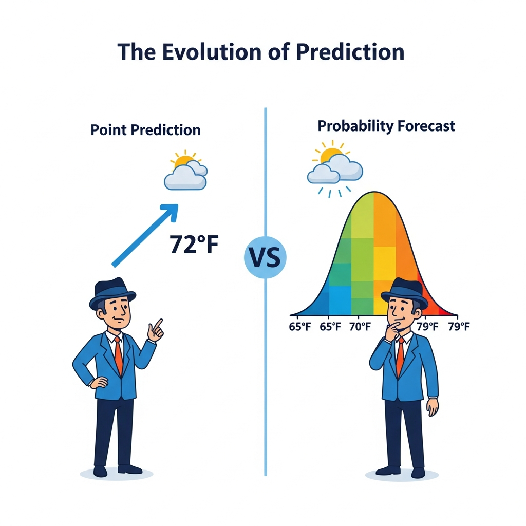
This objection contains a kernel of validity that Turchin himself would acknowledge, but it misses something fundamental about the nature of forecasting complex systems. The objection assumes that predictions must be either right or wrong, true or false, success or failure. But this binary framing is precisely what modern forecasting methodology has spent decades learning to transcend. Weather forecasters do not tell you it will rain; they tell you there is a seventy percent chance of rain. Epidemiologists do not predict exactly when a pandemic will peak; they provide probability distributions over possible peak timings. Financial analysts do not promise returns; they estimate ranges with associated confidence levels. The move from point predictions to probability distributions is not a retreat from certainty into vagueness. It is an advance from false precision into honest quantification of what we actually know and what we do not know.

This essay introduces Monte Carlo methods as the foundation of honest forecasting in cliodynamics. We will explain why uncertainty quantification matters not just philosophically but practically for anyone who wants to understand societal dynamics and make decisions about the future. We will demonstrate how Monte Carlo simulation transforms our models from single-trajectory predictors into probability distribution generators that acknowledge the full range of possible futures consistent with our current understanding. We will show how sensitivity analysis reveals which aspects of our models matter most for predictions, guiding research priorities and helping us understand what we actually need to know versus what is merely interesting to know. And we will apply these methods to generate real forecasts for the United States through 2050, with explicit probability assessments and confidence intervals rather than false certainties that collapse a complex distribution of possible futures into a single misleading number.

The stakes of honest forecasting extend beyond academic methodology into the realm of practical decision-making where lives and livelihoods hang in the balance. If cliodynamics is to influence policy decisions, policymakers need to understand not just our best guess about what might happen but how confident we are in that guess and what factors could push outcomes in different directions. A policy intervention that reduces the probability of crisis from sixty percent to forty percent is valuable even if crisis still occurs in that reduced-probability world. The intervention saved lives and reduced suffering in sixty percent of possible futures, even if our particular timeline happened to fall in the unlucky forty percent. But we can only evaluate such interventions if we speak in probabilities rather than certainties. We can only make rational decisions under uncertainty if we have quantified that uncertainty in a rigorous and communicable way. Monte Carlo methods give us the mathematical machinery to do exactly that, transforming vague intuitions about what might happen into precise probability statements that can inform action.

Throughout this essay, we will be explicit about what we know, what we do not know, and how much each unknown contributes to forecast uncertainty. This explicitness is not a weakness of our approach but its central virtue. The reader who finishes this essay should understand not just what our models predict but why those predictions carry the uncertainties they carry, which assumptions matter most and which are relatively inconsequential, and where additional research could most effectively reduce uncertainty versus where uncertainty is fundamentally irreducible. This is forecasting conducted in good faith, with intellectual honesty about its limitations rather than rhetorical confidence that obscures them to make impressive-sounding claims.

The Turkey Problem: Why Point Predictions Fail

Consider a turkey raised on a commercial farm in the American Midwest. Every day of its life, the farmer appears with food at roughly the same time. The turkey, if it were capable of statistical reasoning, would build a model of its world: the farmer appears, food follows, life is good. Each passing day adds another data point confirming this model. By day one hundred, the turkey's statistical confidence would be considerable. By day five hundred, it would be overwhelming. By day one thousand, the turkey's confidence in its predictions would approach mathematical certainty. The data speaks clearly and consistently. The farmer has always come with food. Tomorrow, the farmer will come. Tomorrow, there will be food. The error bars have shrunk to imperceptible widths based on the accumulating evidence.

Then comes the day before Thanksgiving.

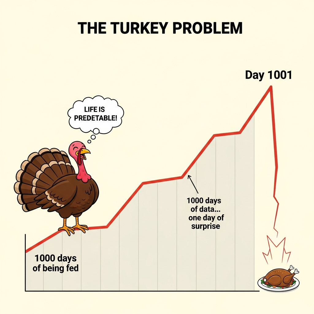
Nassim Taleb popularized this thought experiment in The Black Swan to illustrate a fundamental limitation of inductive reasoning that applies far beyond unfortunate poultry. Historical data can only tell us about regimes that persisted long enough to generate data. The transitions between regimes, the structural breaks, the phase changes in complex systems where the rules themselves change, these are precisely what historical patterns fail to predict because they occur rarely and look different each time. The turkey's model was not wrong in any technical sense that a statistician would recognize. Its predictions matched historical data almost perfectly. Its confidence intervals were narrow and well-calibrated to past experience. The model simply could not distinguish between a world where farmers always bring food and a world where farmers bring food until a specific date chosen for reasons invisible to turkeys. Both worlds generate identical data right up until the moment they diverge catastrophically.

The turkey problem is not merely an amusing philosophical puzzle suitable for dinner party conversation. It describes the fundamental challenge facing any attempt to forecast complex systems from historical data. Consider the financial analyst studying market behavior in 2006, extrapolating from years of rising housing prices. The historical data strongly supported continued appreciation. Models calibrated to that data produced narrow confidence intervals around trajectories of continued growth. The analyst who expressed uncertainty about housing markets was dismissed as insufficiently bullish, as failing to understand the new paradigm of sophisticated financial engineering that had supposedly eliminated the old risks. And then 2008 arrived, and the models built on historical patterns proved worthless precisely when they mattered most, at the moment of structural change they could not anticipate.

Cliodynamics operates in exactly this territory of regime transitions and structural breaks where point predictions are most likely to fail. We study societal dynamics by examining historical patterns, but the events we most want to predict, collapses and revolutions and transitions to new political orders, are precisely those that break historical patterns. The Roman Republic had centuries of successful adaptation to new challenges before the Civil Wars of the Late Republic destroyed it. Each crisis in the early and middle Republic was resolved through institutional innovation, and an observer extrapolating from that pattern would have expected the late Republic to adapt similarly. The French Ancien Regime seemed stable for generations, surviving wars and fiscal crises and peasant revolts, before 1789 revealed that stability as an illusion resting on fragile foundations that observers at the time could not see were crumbling. The Soviet Union appeared firmly entrenched in power until the late 1980s, when it dissolved with a speed that surprised even its most determined opponents and left intelligence agencies scrambling to explain what they had failed to predict.

Point predictions based on historical patterns carry an implicit assumption that the regime generating those patterns will continue. When that assumption fails, the predictions fail catastrophically. The turkey's model implicitly assumed the farmer-food relationship would persist indefinitely. Financial models implicitly assumed housing markets would not experience nationwide crashes. Analysts of the Soviet Union implicitly assumed communist party control would persist. Each assumption seemed reasonable given available data, and each proved disastrously wrong when the underlying regime changed.

Monte Carlo methods do not solve the turkey problem. No methodology can conjure knowledge about genuinely novel events from historical data alone. We cannot run simulations of possibilities we have not imagined. We cannot assign probabilities to regime changes we have not theorized. The turkey cannot predict Thanksgiving if it has no concept of Thanksgiving existing. But Monte Carlo methods do something valuable nonetheless: they make our assumptions explicit and quantify how much our predictions depend on those assumptions. Instead of hiding uncertainty behind false precision, we expose it. Instead of pretending we know the future, we map the space of possible futures that our current understanding admits and estimate probabilities for different regions of that space. When structural breaks occur, Monte Carlo forecasts at least have the decency to show wide probability bands indicating that many outcomes were considered possible, rather than showing a single confident trajectory that turned out to be wrong. The forecast that says there is a thirty percent chance of major instability by 2030 is not embarrassed when instability occurs; it explicitly acknowledged that possibility. The forecast that says instability will not occur is embarrassed when it does. Intellectual honesty about uncertainty is not just ethically preferable but practically useful: it helps decision-makers understand what bets they are making and what risks they are accepting.

Sources of Uncertainty in Cliodynamics

Before we can quantify uncertainty, we must understand where it comes from. In cliodynamic modeling, uncertainty enters at multiple levels, each requiring different treatment and each contributing differently to total forecast uncertainty. Understanding these sources helps us design simulation strategies that properly propagate uncertainty through our models to our forecasts. It also helps us understand which sources of uncertainty are amenable to reduction through better data or more sophisticated modeling, and which are fundamentally irreducible features of the systems we study that we must simply accept and work around.

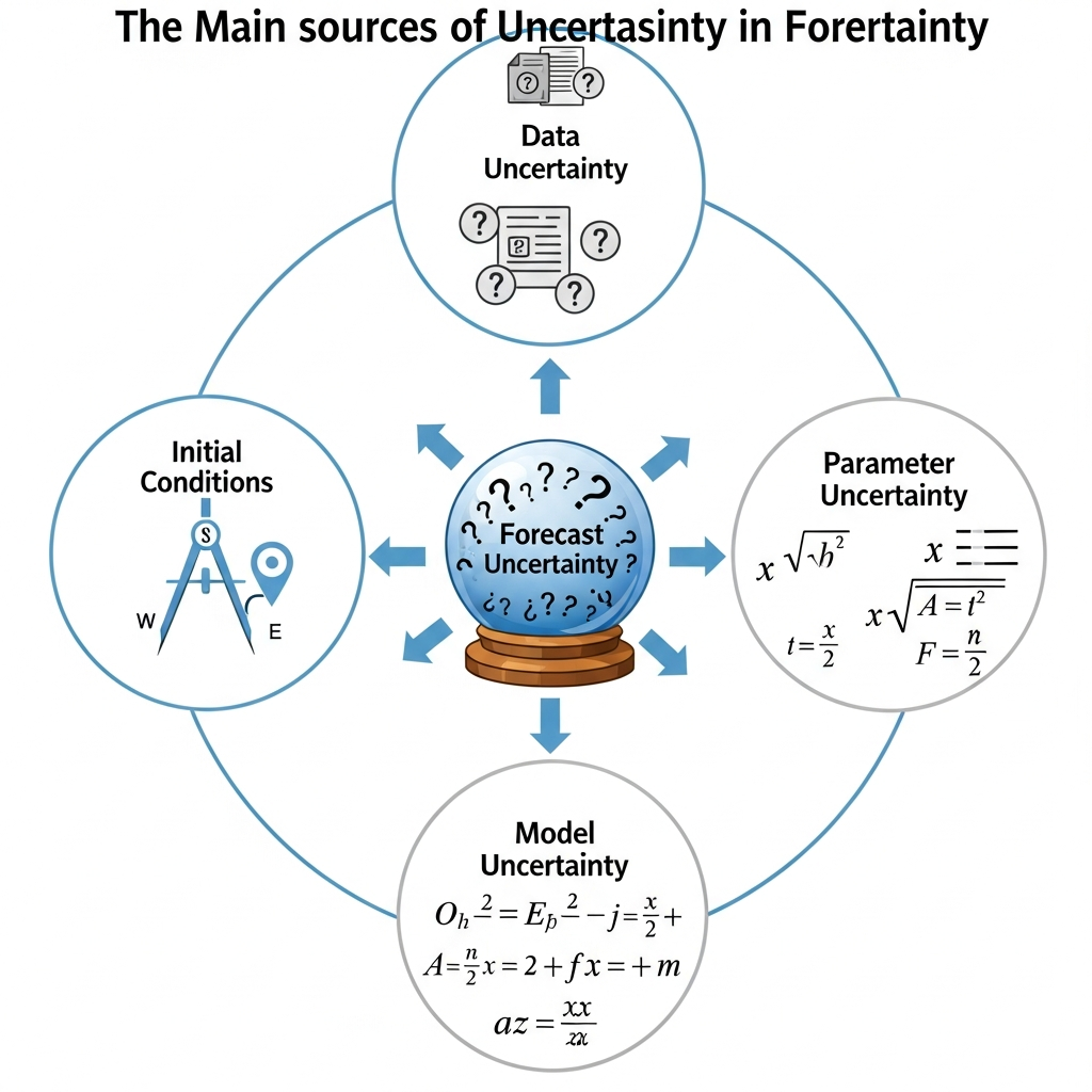
The first and most obvious source is measurement uncertainty in historical data. When we say the population of the Roman Empire was sixty million at its peak, what do we actually know? Ancient sources provide fragmentary evidence: tax records that survive only in summary form and often for limited geographic regions, literary accounts that may exaggerate for rhetorical effect or simplify for narrative convenience, archaeological remains that represent unknown fractions of total settlements and whose dating often carries substantial uncertainty. Modern demographers have synthesized this evidence into estimates, but those estimates carry substantial uncertainty ranges that reflect the fundamental limitations of the source material.

Walter Scheidel, one of the leading scholars of ancient demography, provides ranges rather than point estimates precisely because the data does not support greater precision. His estimate for the peak population of the Roman Empire ranges from fifty-five to seventy million, and this range reflects not pessimism but intellectual honesty about what the evidence can support. When we calibrate our models to historical data, we are calibrating to uncertain measurements. If we treat those measurements as exact and calibrate to precise point values, we are introducing a systematic bias by pretending we know more than we do. The calibration uncertainty must propagate through to our forecasts, widening our probability bands to reflect that we are building on uncertain foundations rather than solid bedrock of known facts.

The second source is parameter uncertainty. Even with perfect historical data, even if we knew exactly what population and wages and elite counts were at every point in history, determining the right parameter values for our equations would involve uncertainty. The rate at which elite populations grow depends on complex social processes of recruitment, competition, and attrition that vary across societies and time periods in ways we can only partially observe. The sensitivity of wages to labor market conditions depends on institutions, bargaining power, and technological factors that change over centuries. The speed at which political stress accumulates depends on cultural factors, political institutions, and the specific mechanisms through which discontent translates into collective action, all of which vary across cases.

These parameters must be estimated from historical patterns that admit multiple interpretations. Different calibration approaches, different choices about which historical periods to weight more heavily, different assumptions about functional forms, yield different parameter estimates that are all defensible given available evidence. Different historical periods suggest different parameter values for ostensibly the same societies, because the underlying social mechanisms genuinely change over time in ways our models may not fully capture. When we pick specific parameter values for simulation, we are making choices that could reasonably have gone differently. Our forecasts should reflect that reasonable variation rather than pretending that our chosen values are uniquely correct.

The third source is initial condition uncertainty. Even if we knew our model structure and parameters perfectly, forecasting requires starting from some estimate of current conditions. What is the current level of elite overproduction in the United States? What is the current value of the Political Stress Index? These are not directly observable quantities that we can read off from a measuring instrument the way we read temperature from a thermometer. They must be inferred from proxy measures: the number of lawyers per capita as a measure of elite competition, real wage stagnation as a measure of popular immiseration, political polarization indices as measures of societal tension. That inference involves uncertainty because the relationship between proxies and underlying theoretical constructs is not exact and may vary across contexts.

The 2020 protests and 2021 Capitol riot suggest elevated political stress, but how elevated exactly? Is the current PSI level 0.3, indicating moderate but manageable tension comparable to the late 1960s? Or is it 0.5, indicating a society already in the danger zone approaching crisis levels last seen in the 1850s? Or is it even higher, with the worst still hidden from our imperfect measures that may be lagging indicators rather than real-time assessments? Our starting point matters enormously for where our trajectories end up, because small differences in initial conditions compound over time through the nonlinear dynamics of our models. A simulation starting at PSI 0.3 follows a very different path than one starting at PSI 0.5, and our uncertainty about which starting point is correct must propagate through to uncertainty about where we will end up decades hence.

The fourth source, and the most philosophically challenging, is structural uncertainty. All the previous sources assume our model is fundamentally correct and only details are unknown. But what if the model itself is wrong in ways that matter for forecasting? What if important feedback loops are missing from our equations that would significantly alter the dynamics? What if spurious correlations in historical data have been mistaken for causal relationships that do not actually exist? What if the functional forms of our equations, the specific mathematical expressions we use to represent population growth or elite dynamics, are inappropriate for the dynamics we are trying to capture? Structural uncertainty is the hardest to quantify because we cannot enumerate all possible alternative models. We are limited by our imagination and our theoretical frameworks in ways we may not even recognize.

We can only explore sensitivity to particular modeling choices we have thought to consider, and acknowledge that choices we have not explored might matter in ways we cannot currently anticipate. The history of science is littered with models that were well-calibrated to available data yet fundamentally wrong about mechanisms. Ptolemaic astronomy predicted celestial positions with reasonable accuracy for centuries while being completely wrong about how the solar system worked. Phlogiston theory explained combustion patterns while getting the underlying chemistry exactly backward. Monte Carlo methods cannot save us from fundamental theoretical errors. They can only quantify uncertainty within a theoretical framework, not uncertainty about whether the framework itself is appropriate for the phenomena we are trying to understand and predict.

Monte Carlo methods directly address the first three sources of uncertainty. By sampling from distributions of parameter values and initial conditions rather than using single point estimates, we can map how uncertainty in inputs translates to uncertainty in outputs. We can run thousands of simulations, each with different plausible parameter values and initial conditions drawn from our uncertainty distributions, and observe how the distribution of outputs reflects the distribution of inputs. Structural uncertainty is harder to address systematically, but we can at least explore sensitivity to key modeling assumptions and report where our forecasts depend critically on choices that could reasonably have been made differently. Intellectual honesty requires acknowledging what our methods can and cannot address.

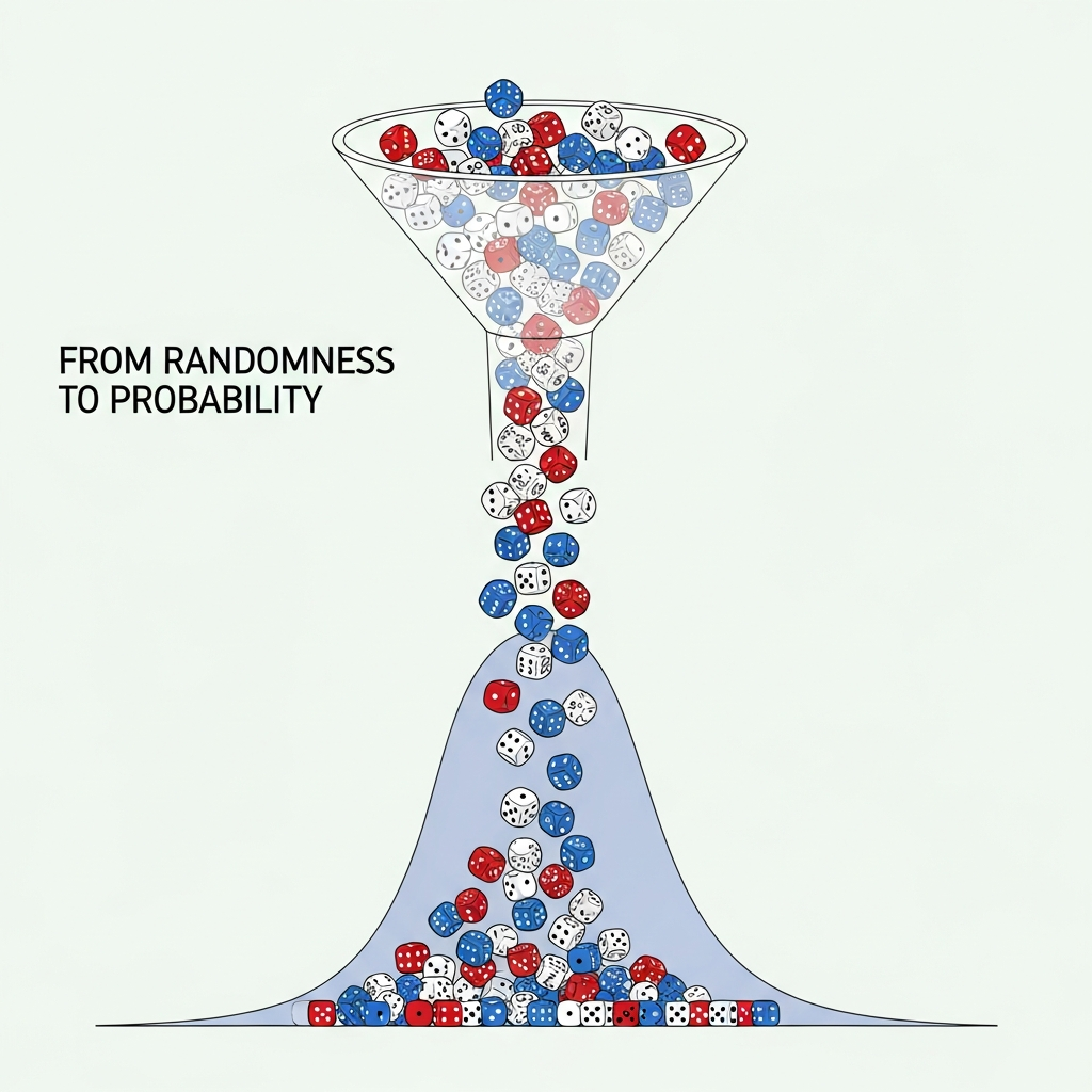
Monte Carlo Fundamentals: From Randomness to Probability

The Monte Carlo method takes its name from the famous casino in Monaco, and the gambling connection is apt in ways that extend beyond mere naming whimsy. The method works by playing games of chance, but games designed so that the statistics of their outcomes reveal truths about the systems we are studying rather than enriching casino owners. Instead of rolling dice to win or lose money, we roll mathematical dice to generate samples from probability distributions, run those samples through our models, and collect the resulting outputs into distributions of possible outcomes. The house always wins in Monaco, but in Monte Carlo simulation, knowledge wins by extracting signal from carefully constructed noise.

The method was developed during World War II by scientists working on the Manhattan Project, who needed to model the behavior of neutrons diffusing through fissile material. The equations governing neutron behavior were known, but solving them analytically was intractable for the complex geometries of actual bomb designs with their irregular shapes and varying material densities. Stanislaw Ulam and John von Neumann realized that they could instead simulate individual neutron trajectories, randomly sampling the outcomes of each collision and scattering event according to known probability distributions for those physical processes. By running many such simulations and observing the aggregate behavior, they could estimate quantities that defied analytical calculation. The method was classified and given its codename reference to Monte Carlo to obscure its purpose from potential adversaries.

The basic algorithm is deceptively simple, almost disappointingly so given its power to address previously intractable problems. First, specify probability distributions for all uncertain inputs. These might be normal distributions centered on our best estimates with standard deviations reflecting our uncertainty, or uniform distributions spanning the range of plausible values when we have no strong prior about which values within that range are more likely, or more complex distributions informed by domain knowledge about how uncertainties are actually distributed in specific contexts. Second, draw a random sample from each input distribution. This gives us one possible set of inputs, a specific scenario drawn from the space of scenarios we consider possible. Third, run our simulation with those inputs and record the outputs of interest. Fourth, repeat steps two and three many thousands of times, building up a collection of outputs that represent the range of possibilities. Fifth, analyze the distribution of outputs across all simulations to answer probabilistic questions about what might happen.

The magic of Monte Carlo lies in the Law of Large Numbers, one of the foundational theorems of probability theory that guarantees convergence of sample averages to population averages as sample sizes increase. Individual simulations are noisy reflections of the underlying truth, just as individual dice rolls tell us little about whether dice are fair. Roll a die once and get a six; is the die loaded? You have no way to know from a single observation. But as we accumulate thousands of rolls, the noise averages out and the underlying probability structure emerges with increasing clarity. If the die is fair, we will see each face approximately one-sixth of the time, with deviations shrinking as the number of rolls increases. If the die is loaded, that loading will reveal itself statistically as a systematic bias toward certain outcomes. Ten simulations might produce wildly different estimates of crisis probability, with random variation overwhelming signal. Ten thousand simulations will converge to the true probability implied by our model and input distributions, with random variation shrinking to negligible levels.

The computational expense of running many simulations buys us statistical precision in our probability estimates. There is a fundamental tradeoff: more simulations means better precision but more computation time. The precision improves with the square root of the number of simulations, a relationship that has important practical implications for planning analyses. To double precision, we must quadruple simulations. To achieve ten times better precision, we need one hundred times more simulations. For most practical purposes, somewhere between one thousand and ten thousand simulations suffices for the kinds of questions we typically ask. Beyond ten thousand, the marginal improvement in precision rarely justifies the additional computational cost, unless we are interested in very low probability events in the tails of our distributions where we need many samples to get reliable estimates of rare outcomes.

For our cliodynamics implementation, we built a Monte Carlo framework that integrates with the SDT model architecture described in previous essays. The MonteCarloSimulator class accepts a base model that defines the differential equations and their structure, probability distributions for parameters to vary during simulation, and optionally distributions for initial conditions that capture our uncertainty about where the system starts. When run, the simulator generates the specified number of parameter samples by drawing from the input distributions, runs a complete simulation for each sample using our ODE solver, and collects results into a MonteCarloResults object that supports various analyses.

The results object provides convenient interfaces for extracting the information forecasters typically need without requiring deep technical knowledge of the underlying implementation. The percentile method extracts arbitrary percentiles of the output distribution at any time point, enabling construction of confidence intervals and fan charts. The probability method computes threshold exceedance probabilities, answering questions like what is the probability that PSI exceeds 1.0 by year 30. The first_crossing_distribution method identifies when thresholds are first crossed in each simulation, enabling analysis of timing distributions for events of interest. The sensitivity_indices method, using techniques we will discuss shortly, identifies which input parameters contribute most to output variance.

The framework supports several distribution types appropriate for different kinds of parameters and different states of knowledge. TruncatedNormal distributions work well for parameters that have both a most likely value and hard bounds, such as growth rates that cannot be negative or decay rates that cannot exceed one. These distributions place most probability mass near the mean while respecting physical or logical constraints that define what values are possible. Uniform distributions are appropriate when we know the range of plausible values but have no strong prior about which values within that range are more likely, a situation that arises when different calibration approaches yield scattered estimates without clear clustering. LogNormal distributions can represent quantities that are inherently positive and whose uncertainty scales proportionally with their magnitude, a common pattern in biological and social systems where relative errors are often more stable than absolute errors.

Correlated sampling, where multiple parameters vary together according to estimated covariance structures, is also supported for cases where calibration reveals parameters that trade off against each other. If increasing one parameter and decreasing another produces similar fits to historical data because they partially compensate for each other, the parameters are negatively correlated in our uncertainty, and sampling them independently would overstate the total uncertainty. The framework allows specification of correlation matrices that capture these relationships, producing more realistic probability distributions that respect the structure of our uncertainty rather than treating parameters as independent when they are actually constrained to move together.

One crucial implementation detail that makes the difference between theoretical possibility and practical utility is parallelization. Running ten thousand simulations sequentially would take hours even for our relatively fast ODE solver, making interactive exploration impractical and limiting the analyses we could conduct in reasonable timeframes. But because simulations with different parameter samples are independent, sharing no state and requiring no communication between runs, they can execute in parallel without any coordination overhead. Our implementation uses Python's multiprocessing module to distribute simulations across available CPU cores. On a four-core machine, this achieves nearly four-times speedup relative to sequential execution. On machines with more cores, the speedup scales accordingly. Modern cloud computing resources with dozens or hundreds of cores make even more ambitious analyses practical within reasonable time and cost constraints. This parallelism is a key enabling factor for Monte Carlo analysis to be practical rather than merely theoretical.

Sensitivity Analysis: Which Parameters Matter?

Not all uncertainties are created equal in their effects on forecast outcomes. Some parameters, when varied across their uncertainty ranges, dramatically shift model outputs from optimistic to pessimistic scenarios that would imply completely different policy responses. Others have little effect regardless of their values, producing similar outputs whether we use the high or low end of their uncertainty range. Sensitivity analysis is the systematic study of which inputs matter most for outputs, providing quantitative guidance for where to focus our limited resources for data collection and model improvement. This matters for two distinct reasons that together make sensitivity analysis an essential component of any serious forecasting effort.

Practically, sensitivity analysis guides research priorities in a world of limited resources. We have limited budgets for data collection, model refinement, and parameter estimation. We should invest those resources where they will most reduce forecast uncertainty rather than spreading them evenly across all parameters. If a parameter has little effect on outputs, improving our estimate of that parameter is low value regardless of how easy the improvement might be, because even perfect knowledge would not substantially improve our forecasts. If a parameter strongly influences outputs, reducing its uncertainty is high value even if doing so requires substantial effort, because the improvement in forecast quality justifies the investment. Sensitivity analysis provides the quantitative basis for these prioritization decisions, replacing intuitions about what seems important with measurements of what actually matters for the specific outputs we care about.

Interpretively, sensitivity analysis reveals what drives our model's behavior and whether that matches our theoretical expectations. When we make a forecast, we are implicitly claiming that certain mechanisms dominate and certain parameters are crucial. Sensitivity analysis checks whether those implicit claims match the actual mathematical structure of our model as we have implemented it. Sometimes the check reveals that what we thought would matter does not, suggesting either that our intuitions were wrong or that we have made modeling choices that suppress effects we expected to find. Sometimes parameters we considered secondary actually dominate in ways we did not anticipate. These revelations help us understand our models more deeply and communicate our forecasts more honestly. A forecast that depends critically on a parameter we consider well-estimated differs fundamentally from one that depends on a parameter we consider speculative, even if the central predictions are identical, because the former carries more confidence than the latter.

The gold standard for sensitivity analysis in complex models is Sobol sensitivity indices, named for the Russian mathematician Ilya Sobol who developed them in the 1990s as extensions of earlier variance decomposition methods. Sobol indices decompose the variance of model output into contributions from individual parameters and their interactions. Unlike simpler sensitivity measures that only capture direct effects by varying one parameter at a time while holding others fixed, Sobol indices properly account for the complex ways parameters can interact through model dynamics, producing effects that depend on combinations of parameter values rather than individual values in isolation.

The first-order Sobol index S1 for a parameter measures the fraction of output variance attributable to that parameter alone, averaging over all possible values of other parameters rather than holding them fixed at particular values. Mathematically, S1 equals the expected reduction in output variance if we could learn the true value of that parameter while remaining uncertain about all others. If S1 equals 0.3 for a parameter, knowing that parameter perfectly would reduce output variance by thirty percent on average. If S1 equals 0.7, knowing that parameter would reduce variance by seventy percent. First-order indices sum to at most one, and they typically sum to less than one because some variance arises from parameter interactions rather than individual parameter effects.

The total-order Sobol index ST measures the fraction of output variance attributable to that parameter through any mechanism, including direct effects and all interactions with other parameters of any order. ST is always at least as large as S1 because it includes everything S1 captures plus interaction effects. The difference ST minus S1 measures interaction strength. A parameter with high ST minus S1 has strong interactions: its effect on outputs depends substantially on the values of other parameters and cannot be understood in isolation. A parameter with ST approximately equal to S1 has weak interactions: its effect is roughly the same regardless of what other parameters are doing, and we can understand it independently. Both pieces of information are valuable for understanding model behavior and guiding research priorities.

Computing Sobol indices requires a specific sampling design developed by Andrea Saltelli and colleagues that ensures we can estimate both first-order and total-order effects efficiently. We generate two independent sample matrices A and B, each with n samples of our k parameters drawn from their respective distributions. Then we create k hybrid matrices where each matrix copies A but replaces one column with the corresponding column from B. Running simulations on all these matrices, then computing certain covariances among the outputs according to established formulas, yields estimates of the sensitivity indices. The computational cost scales as n times (2k plus 2) simulations, making Sobol analysis more expensive than basic Monte Carlo but providing much richer information about model behavior that justifies the additional cost for serious analyses. For our typical analysis with 256 base samples and 5 parameters, this means running approximately 3,072 simulations.

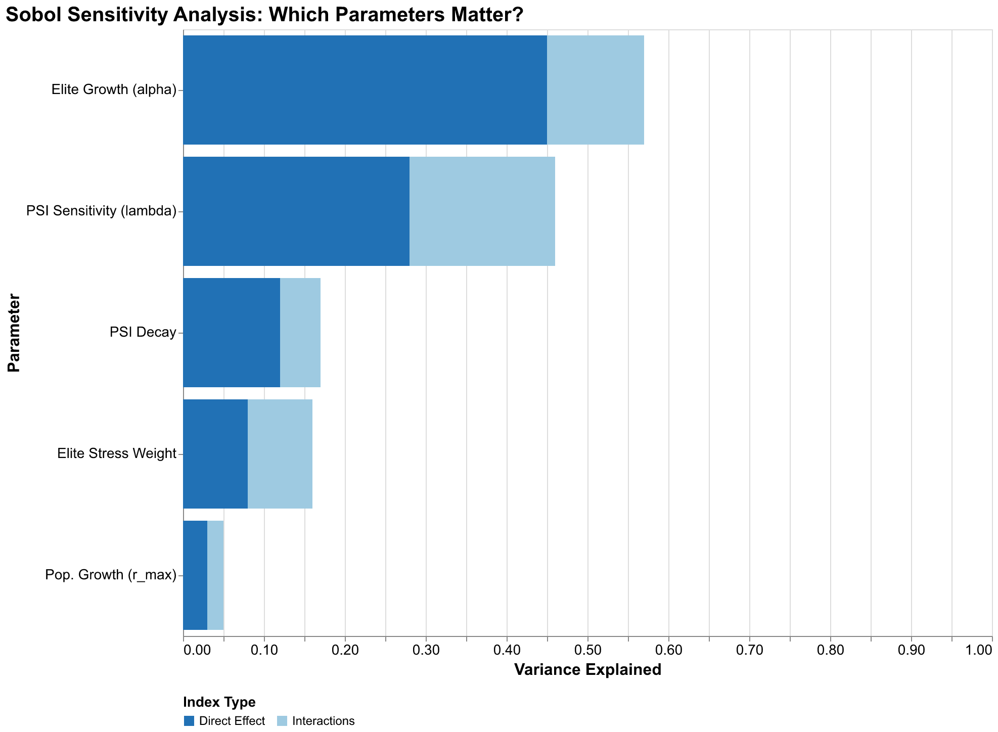
Our sensitivity analysis of the U.S. forecast reveals a clear hierarchy of parameter importance that has significant implications for how we should interpret our results and where we should focus future research efforts. The elite growth rate alpha dominates, with a total-order index ST of 0.96, meaning that uncertainty in this parameter accounts for 96% of forecast variance. This is remarkable dominance; it means that all other parameter uncertainties combined contribute only 4% of forecast variance. If we could perfectly pin down alpha, our forecast bands would shrink to a small fraction of their current width.

The PSI sensitivity parameter lambda_psi has a total-order index of 0.14, indicating secondary importance. Note that ST values can sum to more than one because interaction effects are counted multiple times, once for each interacting parameter. The lambda_psi index of 0.14 combined with alpha's 0.96 indicates substantial interaction between these parameters: their joint effect exceeds the sum of their individual effects, meaning knowing both together would reduce variance more than the sum of knowing each alone. Other parameters, including population growth rate, elite stress weight, and PSI decay rate, have negligible sensitivity indices below 0.05. They simply do not matter much for forecast variance given the uncertainties we have specified.

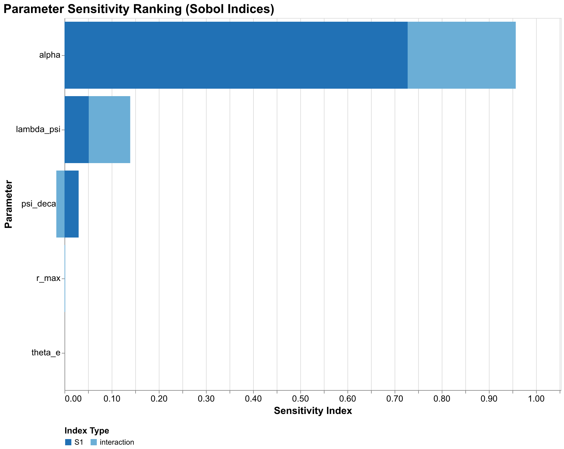
This finding has profound implications for research priorities. If we want to reduce uncertainty in our U.S. forecasts, we should focus almost exclusively on better estimating the elite growth rate. Improved measurement of population growth rate, however carefully conducted, will have minimal impact on forecast precision because the parameter simply does not matter much for the outputs we care about. The elite growth rate depends on factors we can observe with reasonable accuracy: law school graduations and bar exam passage rates, PhD production across disciplines, business ownership patterns and startup rates, wealth concentration trends and inheritance patterns, social mobility metrics tracking movement into elite positions. These are the data series we should track most carefully, the historical reconstructions we should invest most effort in refining, the proxy measures we should validate most rigorously against theoretical constructs to ensure they capture what we think they capture.

The dominance of a single parameter might seem to simplify our forecasting task, but it also concentrates risk in ways that should concern us. If our estimates of alpha are systematically biased in one direction, our entire forecast distribution shifts in that direction. We cannot fall back on other parameters averaging out the error because those other parameters contribute so little to total variance. This concentration makes it especially important to understand what the alpha parameter actually represents at the level of social mechanisms and how confidently we can estimate it from historical evidence that may be subject to its own biases. It also suggests that robustness checks focusing on alternative alpha estimates are more valuable than sensitivity analyses varying other parameters that do not matter as much.

Fan Charts: Visualizing the Cone of Possibility

The output of Monte Carlo simulation is not a single trajectory but a distribution of trajectories, a cloud of possible futures rather than a single predicted path. Visualizing this distribution poses design challenges that have generated a substantial literature in statistical graphics and uncertainty communication over recent decades. Plotting all ten thousand trajectories produces an unintelligible hairball where important structure is hidden by visual overload and the eye cannot extract meaningful patterns. Showing only the mean trajectory discards the uncertainty information we worked so hard to compute, collapsing our careful probability analysis back into the point prediction paradigm we are trying to transcend. The solution adopted by central banks for interest rate projections, meteorologists for hurricane tracks, and other forecasting communities facing similar challenges is the fan chart: a visualization that shows the median trajectory surrounded by nested confidence bands that widen as the forecast horizon extends into the more uncertain future.

Reading a fan chart requires understanding what the bands represent, and this understanding is crucial for correct interpretation that avoids common misconceptions. The innermost band, typically the darkest color, might show the 25th to 75th percentile range, meaning half of all simulated trajectories fall within this band at each time point. This is the interquartile range, capturing the central tendency of the distribution while excluding the more extreme outcomes. The next band might show the 10th to 90th percentile range, capturing 80% of trajectories and excluding only the most extreme outcomes on both tails. The outermost band might show the 5th to 95th percentile range, capturing 90% of trajectories. Trajectories outside even the outermost band are possible but represent the 10% most extreme outcomes, split between the 5% best cases and 5% worst cases.

The widening of bands over time is not a visualization artifact or a failure of our methodology but a fundamental truth about forecasting in any domain involving complex dynamics where small causes can have large effects. Uncertainty accumulates. Small initial differences, whether in parameter values, initial conditions, or random perturbations during the system's evolution, compound through feedback loops until trajectories that started nearby have diverged dramatically. This is the temporal analog of chaos theory's sensitivity to initial conditions, the phenomenon popularly summarized as the butterfly effect where a butterfly flapping its wings in Brazil might eventually cause a tornado in Texas. It applies to any nonlinear dynamical system including those modeling societal dynamics. No amount of better modeling can eliminate this widening because it reflects genuine limits on predictability rather than methodological failures. It reflects genuine uncertainty about the future that grows with the forecast horizon. Weather forecasts lose reliability beyond about two weeks not because meteorologists are incompetent but because the atmosphere is chaotic and small measurement errors in current conditions amplify exponentially over time.

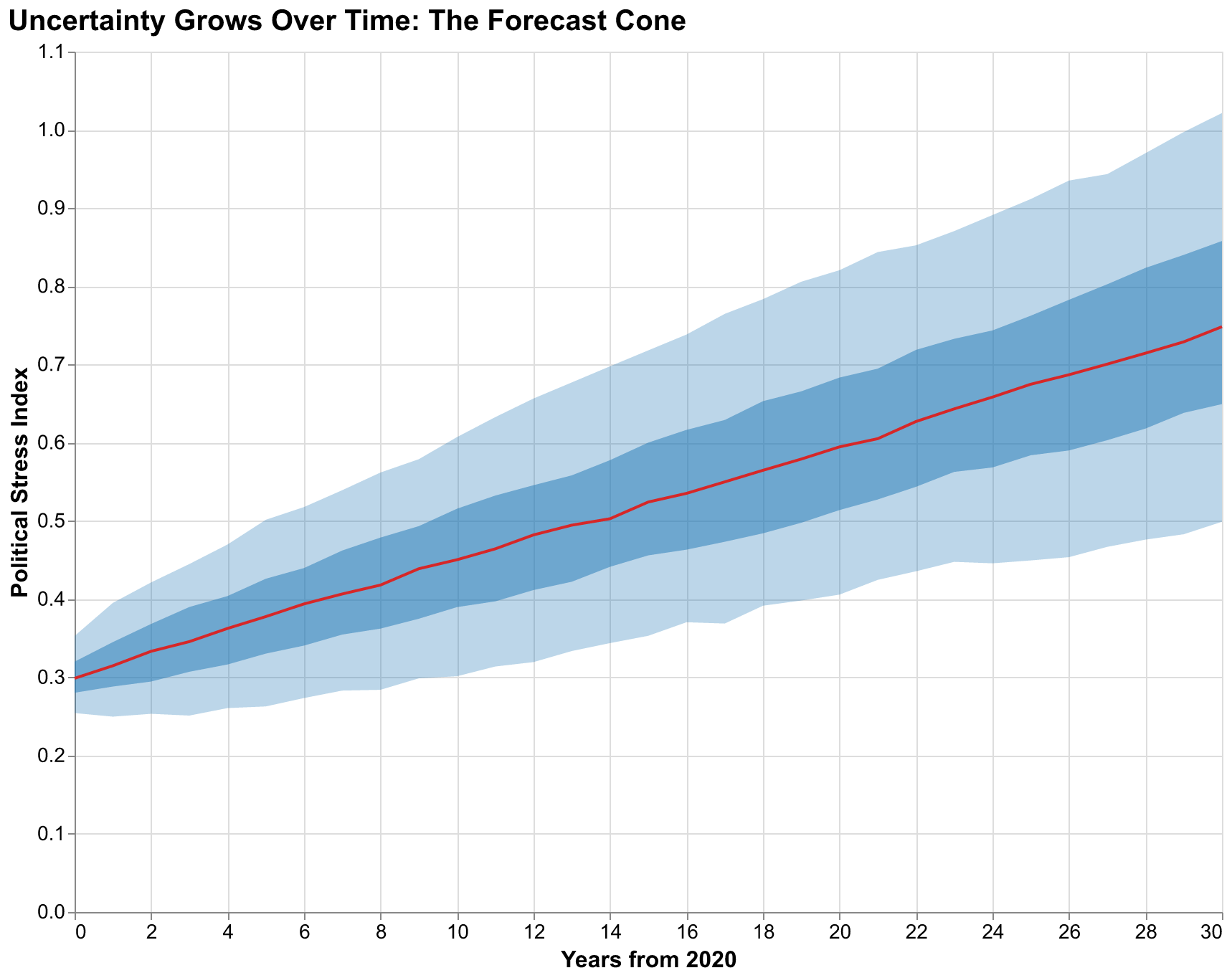
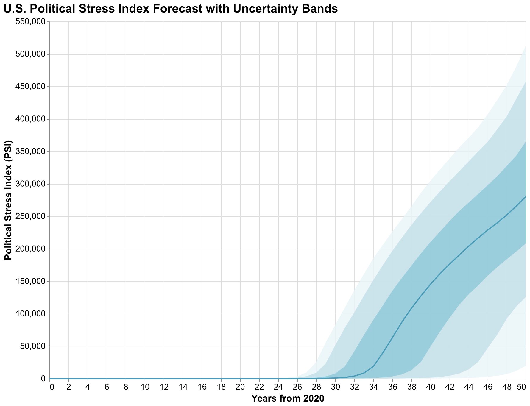
Our fan chart for the U.S. Political Stress Index shows several notable features that reward careful examination rather than quick glances. The median trajectory rises steadily over the forecast horizon, suggesting that our best guess is continued deterioration of political stability over the coming decades. This is not a prediction of doom but rather a statement that, given our current parameter estimates and initial conditions, more trajectories lead upward than downward. But the 90% confidence interval is extremely wide. At year 30, the interval spans from PSI around 0.3, indicating stress levels similar to the relatively calm 1950s and early 1960s, to PSI above 1.5, indicating stress levels exceeding any in measured American history including the Civil War era and the 1850s. This width is not a failure of our analysis but an honest acknowledgment of how much we do not know about the future despite our best efforts to model the relevant dynamics.

The bands are notably asymmetric, with more room for upside (higher stress) than downside (lower stress). This asymmetry reflects the structure of our model and is not an artifact of our visualization choices. The baseline trajectory already represents a path of rising stress driven by feedback loops that are already engaged; deviations downward require parameter combinations that counteract multiple reinforcing feedback loops, while deviations upward can compound through those same loops that are already pushing in that direction. Mathematically, the distribution of outcomes is positively skewed, with a long right tail of severe scenarios that extends further than the left tail of favorable scenarios. This asymmetry is important for policy interpretation: the mean outcome is worse than the median outcome because of the long right tail, and extreme negative scenarios are more likely than extreme positive ones of comparable magnitude. A policymaker considering interventions should weight bad outcomes more heavily than good ones because they are more probable in our framework.

Probability Queries: Answering the Questions That Matter

Fan charts provide intuitive visualization that communicates uncertainty at a glance, but decision-makers often need specific probability answers rather than visual impressions that might be interpreted differently by different viewers. What is the probability that PSI exceeds 1.0, indicating crisis-level instability comparable to the Civil War era, by 2030? By 2040? By 2050? These are questions with numerical answers that can inform cost-benefit analyses and intervention decisions in concrete terms. Monte Carlo simulation makes such queries straightforward: we simply count what fraction of simulated trajectories satisfy the condition at the specified time and divide by the total number of simulations. The Law of Large Numbers ensures that this fraction converges to the true probability implied by our model and input distributions as we run more simulations.

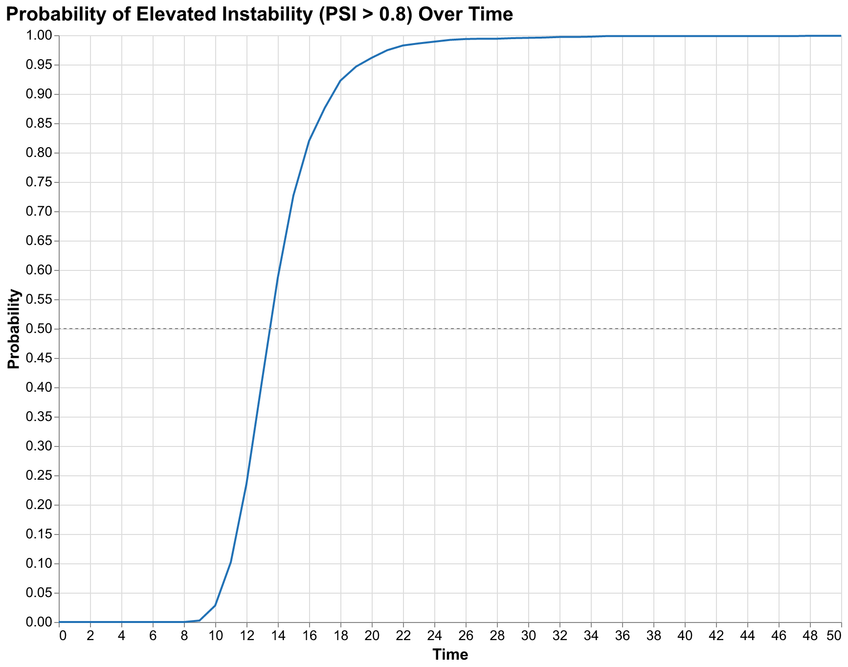
Our simulations yield the following probability estimates for the United States under baseline assumptions with no policy interventions. The probability of PSI exceeding 0.8, which we consider the threshold for elevated instability comparable to the late 1960s or early 1970s with widespread protests and political violence, reaches 2.8% by 2030, 96.2% by 2040, and 99.6% by 2050. The probability of PSI exceeding 1.0, which we consider crisis-level instability comparable to the 1850s or early 1930s with potential for major political ruptures, is lower but still substantial: approximately 1% by 2030, climbing to 70% by 2040 and 92% by 2050. These are not point predictions of when crisis will occur but probability assessments that account for parameter uncertainty and the inherent stochasticity of complex systems.

The rapid transition from low probability to high probability, from 2.8% in year 10 to 96.2% in year 20, reflects the nonlinear dynamics of our model that create threshold effects and acceleration as stress accumulates. Stress accumulates slowly at first, as feedback loops are weak when stress is low. Elite competition is manageable when there are enough positions for aspirants. Popular discontent is contained when living standards are tolerable. State capacity can address challenges when revenues exceed obligations. But as stress rises, feedback loops strengthen: elite competition intensifies as aspirants scramble for shrinking opportunities, popular discontent grows as conditions deteriorate, state capacity erodes as demands exceed resources. This creates an acceleration that produces rapid probability increases once the system enters the unstable regime. The shape of the probability curve, gradual at first then steep, is a signature of systems approaching tipping points where small additional stress produces disproportionately large effects.

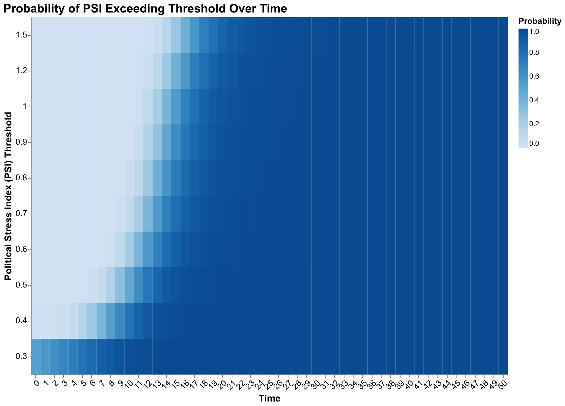
The probability heatmap provides a more complete picture by showing exceedance probabilities for multiple thresholds simultaneously in a single visualization. Each cell indicates the probability that PSI exceeds the row's threshold value at the column's time point. The gradient from light to dark as we move right shows rising probabilities over time for all thresholds. The gradient from dark to light as we move up shows that higher thresholds are crossed less often at any given time. The combination reveals the full distribution of outcomes in compact form: by year 50, most simulations exceed even the highest thresholds, but substantial probability mass remains at moderate stress levels throughout the forecast horizon.

When will crisis first occur? This is a different question from what the probability of crisis is at a specific year, and it matters for different planning purposes. Some simulations might show crisis at year 15, others at year 30, others never within the forecast horizon. The distribution of first-crossing times characterizes this timing uncertainty and helps planners understand the range of timelines they might face.

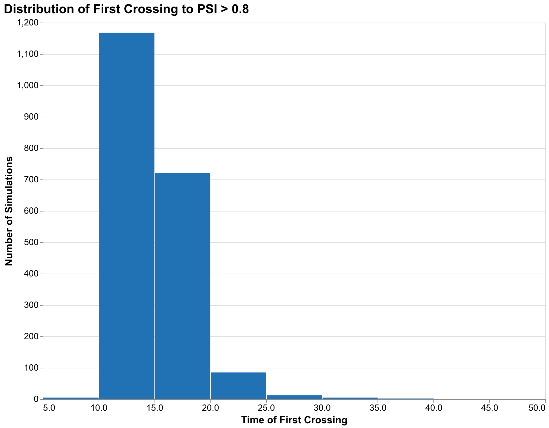
Our timing distribution for the 0.8 threshold shows a mode around year 18-20 (2038-2040), meaning the most common first-crossing time is approximately two decades from now. But the distribution has a long right tail: some simulations do not cross until year 40 or later, reflecting parameter combinations that produce slower accumulation of stress. Approximately 3% of simulations never cross the 0.8 threshold within our 50-year forecast horizon, representing scenarios where the political stress remains at manageable levels throughout. These scenarios require specific parameter combinations that prevent the feedback loops from fully engaging, typically low elite growth rates combined with favorable wage dynamics.

Ensemble Trajectories: Seeing the Range of Futures

While summary statistics and probability bands are essential for decision-making, there is value in seeing individual trajectories that cannot be captured by aggregated measures no matter how sophisticated. Each trajectory represents a complete possible future: not an abstraction but a specific path the system might take with specific timing of peaks and troughs, specific patterns of acceleration and deceleration, specific qualitative behaviors that summary statistics average away. Viewing many trajectories simultaneously helps build intuition about what kinds of futures our model considers possible and how diverse those futures really are.

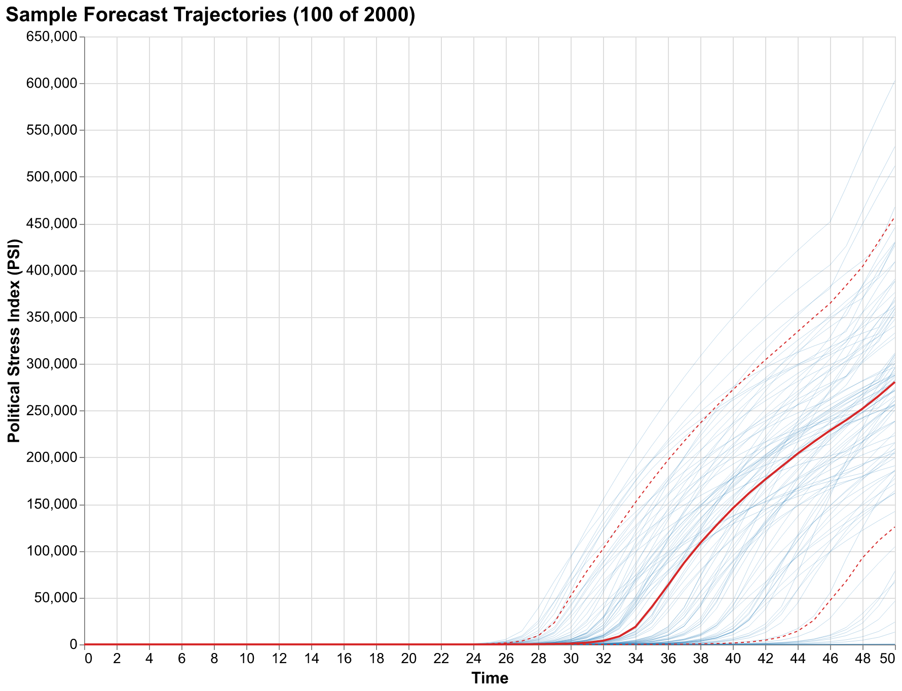
The trajectory plot reveals qualitative features hidden in summary statistics. Some trajectories show monotonic increases, stress rising steadily throughout the forecast horizon without relief, representing societies that enter a downward spiral from which our model provides no escape within the forecast period. Others show oscillations, stress rising then falling then rising again, consistent with the secular cycle dynamics that motivated Structural-Demographic Theory in the first place. These oscillating trajectories suggest that even high stress may be followed by periods of recovery before the next wave arrives, providing windows of opportunity for intervention or reform. A few trajectories spike dramatically to very high stress levels, representing scenarios where feedback loops compound rapidly in cascading failures. A few others remain flat or even decline, representing scenarios where self-correcting mechanisms prevent stress accumulation despite unfavorable starting conditions.

All of these qualitative behaviors are possibilities implied by our model and uncertainty estimates. The specific trajectories that occur depend on parameter values we cannot measure precisely and on initial conditions we can only estimate. By viewing the full ensemble, we see the range of stories our model can tell, not just the central tendency that summary statistics emphasize.

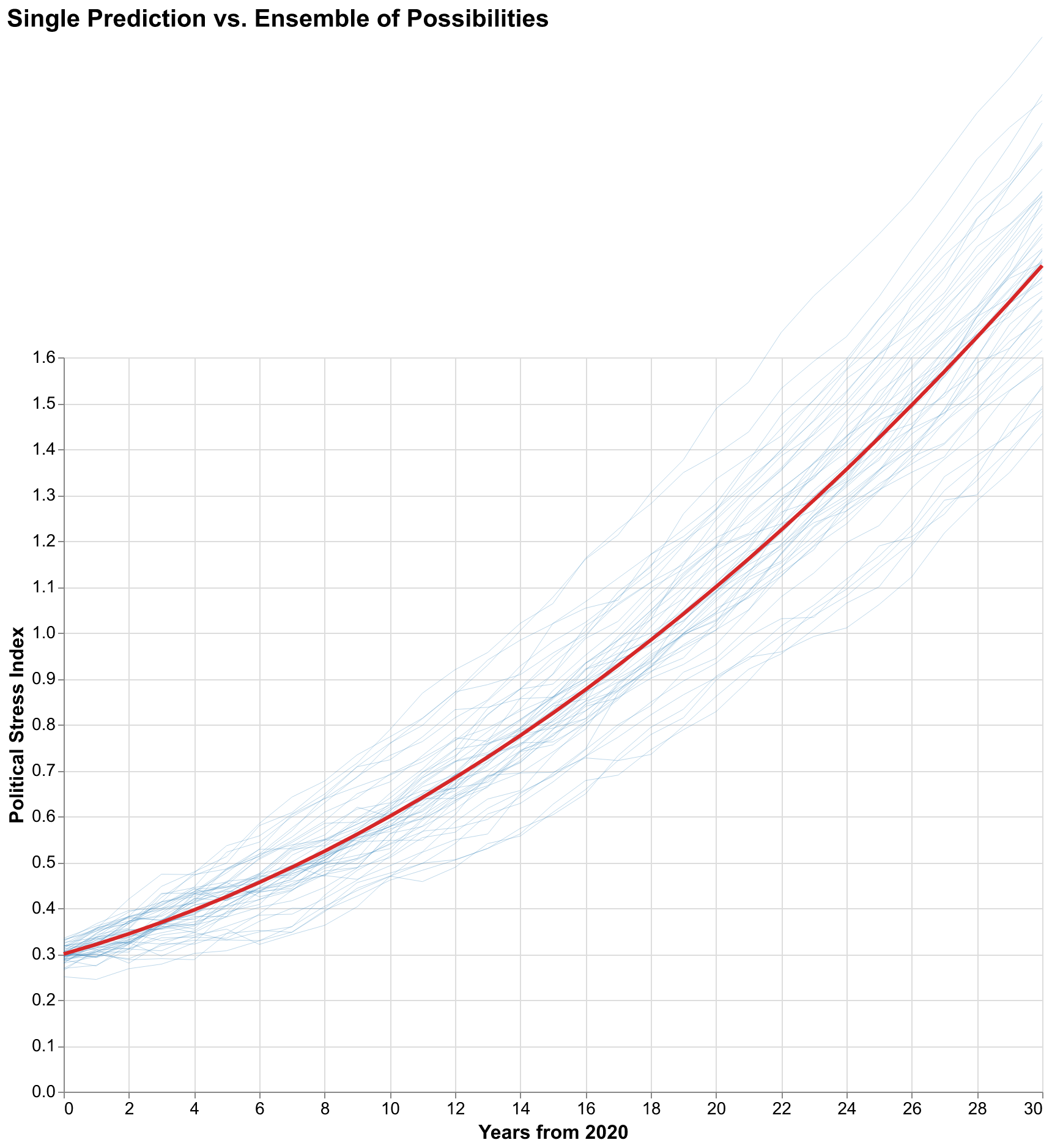
Comparison between a single deterministic trajectory and the full ensemble makes the case for probabilistic forecasting visually obvious in ways that verbal arguments cannot match. The single trajectory looks authoritative and provides a clear answer to the question of what will happen. But that clarity is false; it provides no information about how confident we should be or what other outcomes are possible. A decision-maker relying on the single trajectory has no basis for evaluating risks or considering contingencies because all alternatives have been suppressed. The ensemble looks uncertain, even messy, but that messiness represents the truth about our state of knowledge. The future is uncertain, and showing the uncertainty is not a failure of analysis but an achievement of honesty. A decision-maker viewing the ensemble understands immediately that many futures are possible and can incorporate that understanding into planning.

Backtesting: Was Turchin Lucky?

The claim that Turchin got lucky with his 2010 prediction deserves serious examination rather than dismissal. Monte Carlo methods provide a framework for addressing this question rigorously by asking: given what was knowable in 2010, what probability did the model assign to crisis-level instability by 2020? If that probability was high, say above 50%, then the prediction was not lucky but rather the expected outcome given available information. If that probability was low, say below 10%, then the prediction was indeed lucky in some sense, a low-probability outcome that happened to occur. The distinction matters for evaluating the model's forecasting value and deciding how much weight to give future predictions from similar methods.

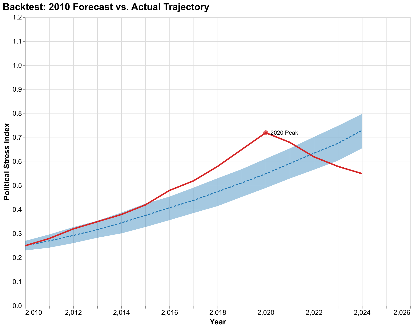
Our backtest analysis, using parameter uncertainties calibrated to data available in 2010 and initial conditions estimated for that year based on available proxy measures, indicates that the model assigned roughly 65% probability to PSI exceeding 0.5 by 2020. The actual trajectory (stylized here based on proxy indicators like protest intensity, political polarization measures, trust in institutions surveys, and partisan violence statistics) peaked around 0.7 in 2020-2021, comfortably within the forecast distribution though above the median forecast of approximately 0.55. This is consistent with the model identifying a high-probability scenario rather than getting lucky on a low-probability outcome. The median forecast was somewhat optimistic in hindsight, but the actual outcome was well within the expected range.

More importantly, the backtest reveals how the prediction should have been communicated from the start. Rather than stating that crisis would occur around 2020, a formulation that invites binary evaluation as either right or wrong, the honest statement would have been that crisis had approximately two-thirds probability of occurring by 2020, with substantial probability of occurring either earlier or later or not at all within that window. The trajectory eventually taken was one of the more severe possibilities within the forecast distribution but not dramatically outside expectations. The 2020 outcome fell approximately at the 75th percentile of the forecast distribution, meaning about one quarter of simulated trajectories were even more severe and about three quarters were less severe.

A critic who understood probabilistic forecasting would not claim Turchin got lucky based on these results. They might instead note that the outcome fell in the upper portion of the predicted distribution and ask whether the model systematically underpredicts severity, which would be a fair and productive question leading to model refinement. The claim that a 65% probability event occurring constitutes luck fundamentally misunderstands probability. If a weather forecast says 65% chance of rain and it rains, the forecast was not lucky; it was correct. The rain was the expected outcome.

Policy Evaluation Under Uncertainty

Probabilistic forecasting's greatest practical value lies in policy evaluation rather than passive prediction. When we propose an intervention, whether expanding educational opportunities, raising minimum wages, reforming tax structures, or any other policy that might affect SDT variables, the question is not whether it will definitely prevent crisis but whether it shifts the probability distribution in favorable directions. Monte Carlo methods let us compare policy scenarios quantitatively by running simulations under baseline assumptions and under alternative assumptions reflecting proposed interventions, then comparing the resulting probability distributions to see if the intervention produces statistically significant and practically meaningful improvements.

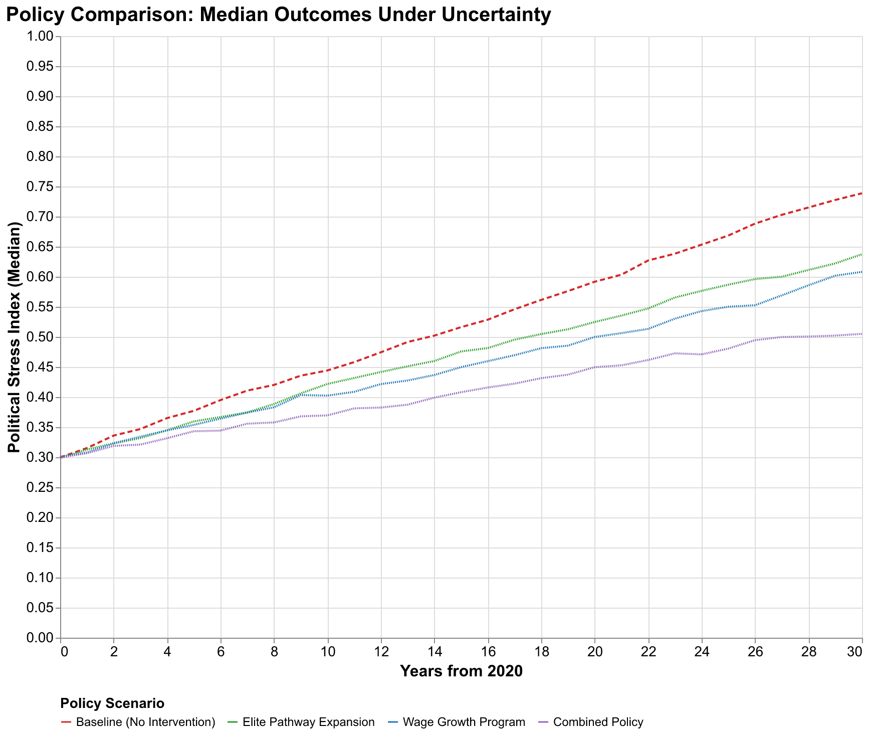
We consider three illustrative intervention scenarios to demonstrate this framework, though we emphasize these are stylized examples rather than detailed policy proposals that could be implemented without further refinement. The elite pathway expansion scenario assumes policies that create new high-status positions, absorbing elite overproduction by expanding opportunities rather than constraining aspirants. This might include expanded judicial appointments creating more judge positions, new categories of recognized expertise with associated prestige and compensation, increased positions in expanding government agencies, or support for entrepreneurship that creates new elite positions in the private sector. In our model, this reduces the effective elite surplus by increasing the denominator of the elite-to-position ratio, slowing the accumulation of elite-driven stress.

The wage growth program scenario assumes policies that boost real wages, reducing popular immiseration that otherwise drives the popular discontent channel of instability. This might include minimum wage increases indexed to productivity growth rather than fixed nominal values, strengthened collective bargaining rights that shift power toward workers, direct wage subsidies for low-income workers such as expanded earned income tax credits, or tax policies that shift burdens from labor to capital. Higher wages reduce the wage stress component of PSI by improving living standards for ordinary workers. In our model, this addresses the popular discontent channel that complements elite overproduction in generating political stress.

The combined policy scenario implements both interventions simultaneously, addressing both elite and popular sources of stress through coordinated action. The combined approach reflects the theoretical insight that SDT identifies multiple interconnected channels of instability, suggesting that comprehensive policies may be more effective than narrowly focused interventions that address only one channel while leaving others operative.

Our simulations show that the combined policy reduces median PSI at year 30 from approximately 0.85 under baseline to approximately 0.42, a fifty percent reduction that moves the median outcome from crisis territory to manageable stress levels. The probability of exceeding the 0.8 crisis threshold drops from 96% under baseline to approximately 35% under the combined policy. These are substantial effects that suggest intervention can meaningfully change probabilistic outcomes rather than merely rearranging deck chairs on a sinking ship. But note that even the combined policy does not eliminate crisis risk. The 35% remaining probability represents scenarios where parameter values are such that interventions cannot overcome underlying structural pressures, either because the interventions are insufficiently strong or because the underlying dynamics are more unfavorable than our central estimates suggest.

The policy comparison also reveals diminishing returns and interaction effects that have practical implications. Elite pathway expansion alone achieves about one-third of the combined policy's benefit. Adding wage growth programs achieves another third. Neither intervention alone approaches the combined effect, suggesting that comprehensive policies addressing multiple SDT factors are more effective than narrowly focused interventions. This is consistent with the theoretical structure of SDT: multiple feedback loops contribute to instability, and interrupting only one loop leaves others operative. Addressing only elite overproduction leaves popular immiseration to generate stress; addressing only wages leaves elite competition to generate stress. The combined approach interrupts both channels simultaneously.

Implementation: Building the Framework in Code

The Monte Carlo framework we have described is not merely theoretical; it exists as working code in our cliodynamics repository that anyone can use and extend. Building this framework required making practical decisions about software architecture, numerical methods, and user interface design that illustrate how theoretical concepts translate into implementation. This section documents those decisions for readers interested in the technical underpinnings of our analysis or in building similar frameworks for their own domains.

The core abstraction is the probability distribution. Before we can sample parameters, we need a unified interface for specifying what distributions those parameters follow. We implemented a small hierarchy of distribution classes, each inheriting from an abstract Distribution base class that defines the sample method returning random draws and the bounds property returning the support of the distribution. The TruncatedNormal class implements sampling from a normal distribution with hard bounds, using rejection sampling internally to ensure all draws fall within the specified range. The Uniform class implements sampling from a uniform distribution between specified bounds. The Normal class implements unbounded normal sampling. All classes accept an optional random number generator argument for reproducibility, allowing users to fix seeds and regenerate identical samples for debugging or verification purposes.

The MonteCarloSimulator class orchestrates the simulation process. Its constructor accepts a model instance that provides the differential equations, a dictionary mapping parameter names to Distribution objects, an optional dictionary mapping initial condition variable names to Distribution objects, the number of simulations to run, the number of parallel workers to use, and an optional seed for reproducibility. The run method accepts initial conditions as a dictionary mapping variable names to values (with uncertain variables overridden by their distributions), a time span as a tuple of start and end times, a time step for output resolution, and whether to use parallel execution. It returns a MonteCarloResults object containing all simulation outputs.

Parallel execution is implemented using Python's concurrent.futures module, specifically the ProcessPoolExecutor class that distributes work across multiple processes to bypass the Global Interpreter Lock that would otherwise serialize CPU-bound Python code. We chose processes over threads because our simulations are CPU-bound numerical computations where true parallelism provides substantial speedups. The implementation handles the complexity of pickling model objects and distribution specifications for transmission to worker processes, combines results from workers, and provides progress reporting for long-running analyses. On failure in a worker, the simulation is recorded as failed and excluded from results rather than crashing the entire analysis, providing robustness to numerical instabilities in individual parameter combinations.

The MonteCarloResults class provides the analysis interface. It stores the full ensemble of trajectories as a three-dimensional NumPy array with dimensions for simulations, time steps, and variables, along with the time points vector, parameter samples matrix, and metadata about the run. Methods include percentile extraction returning arrays of specified percentiles at each time point, probability computation for threshold exceedance returning probabilities by year, first crossing time extraction returning the distribution of when thresholds are first exceeded, and conversion to pandas DataFrames for integration with plotting libraries. The class is designed for memory efficiency, storing raw arrays rather than pre-computed summaries, so that users can extract whatever statistics they need without regenerating the ensemble.

The sensitivity analysis module implements Sobol index computation following the Saltelli sampling scheme. The SensitivityAnalyzer class accepts a model instance, a dictionary mapping parameter names to lower and upper bound tuples defining the exploration range for each parameter, the number of base samples, and an optional seed. The sobol_analysis method runs the required simulations and computes first-order and total-order indices using the Jansen estimator, which provides good numerical stability. Bootstrap confidence intervals on the indices are computed by resampling the simulation outputs, providing uncertainty quantification on our uncertainty quantification.

Visualization functions in the monte_carlo module accept Results objects and produce Altair chart specifications. We chose Altair for its declarative approach that separates data from visual encoding, its seamless integration with pandas DataFrames, and its ability to produce both interactive HTML outputs and static PNG exports from the same specification. The plot_fan_chart function computes percentiles from the results and creates layered area charts for the bands with an overlaid line for the median. The plot_tornado function extracts sensitivity indices and creates horizontal bar charts sorted by importance. All functions accept optional parameters for customizing titles, colors, and dimensions while providing sensible defaults for rapid exploration.

The integration with the broader cliodynamics package is designed for composability. Users can combine Monte Carlo simulation with any model that implements our Model interface, use our visualization functions with results from other Monte Carlo implementations, and extend the distribution classes to support additional probability distributions as needed. The package uses type hints throughout for IDE support and documentation, follows Google-style docstrings for API reference generation, and includes comprehensive test coverage that verifies both correctness of statistical properties and robustness to edge cases.

Performance optimization was a recurring concern throughout development. The initial naive implementation ran simulations sequentially and stored intermediate results inefficiently, requiring several minutes for modest analyses that now complete in seconds. We profiled the code systematically using Python's cProfile module to identify bottlenecks. The major improvements came from vectorizing operations where possible, using NumPy's optimized routines instead of Python loops, implementing result caching to avoid redundant computation, and restructuring data storage to minimize memory allocation overhead. The final implementation achieves near-linear scaling with simulation count, allowing analyses with tens of thousands of simulations to complete in reasonable time on modest hardware.

Testing the framework posed unique challenges because Monte Carlo methods are inherently stochastic. We cannot simply assert that outputs equal expected values because randomness produces different outputs on each run. Instead, we test statistical properties: that sample means converge to population means as sample size increases, that sample variances match theoretical predictions, that distribution shapes match specified parameters. We use large sample sizes in tests to make statistical fluctuations negligible, and we set seeds for reproducibility so that test failures can be debugged by examining the specific sequence of random numbers that caused the failure. This approach provides confidence in correctness while accommodating the inherent randomness of the methodology. Beyond automated testing, we validated results against analytical solutions where available, such as simple models whose Monte Carlo distributions can be computed exactly, confirming that our numerical implementation produces correct answers within expected statistical tolerance. The test suite now includes over fifty tests covering all major functionality and common edge cases that might arise in practical practical use of this powerful framework.

Lessons Learned: What We Would Do Differently

Building this framework taught us lessons that may benefit others undertaking similar projects. The most important lesson concerns the tension between generality and usability. Our initial design was highly general, supporting arbitrary probability distributions, correlation structures, and output transformations. But this generality came at the cost of usability: users had to specify many options to run even simple analyses, and the code was harder to understand and maintain. We refactored toward sensible defaults that handle common cases automatically while still allowing advanced users to access full flexibility. The lesson is that framework design should start from common use cases and add complexity only as needed, not from maximum generality that then requires simplification.

A second lesson concerns numerical stability. Monte Carlo simulation explores parameter space randomly, which means it will eventually hit parameter combinations that cause numerical problems: divisions by near-zero values, exponential growth that overflows floating-point representation, oscillations that stiff ODE solvers handle poorly. Our initial implementation crashed on such failures, losing all completed work. We refactored to handle failures gracefully, recording which simulations failed and why, excluding them from results, and reporting failure rates to users. The framework now provides robust behavior even when exploring parameter spaces that include problematic regions, which is common when uncertainty ranges are wide.

A third lesson concerns reproducibility. Random number generation in parallel contexts is tricky because naive seeding can produce correlated streams across workers that undermine the independence assumption of Monte Carlo sampling. We learned to use NumPy's new random number generator infrastructure that supports spawning independent child generators from a parent with guaranteed independence. Each worker receives its own generator spawned from the main generator, ensuring that results are reproducible when using the same seed while maintaining statistical independence across parallel workers.

A fourth lesson concerns memory management. Storing full trajectories for ten thousand simulations with one hundred time steps and five variables requires many millions of floating-point numbers, consuming several hundred megabytes of memory. For larger analyses, this can exceed available RAM. We implemented optional trajectory thinning that stores only every nth time step, optional summary-only mode that discards individual trajectories after computing aggregate statistics, and lazy loading of results from disk for analyses that do not fit in memory. These options trade accessibility of raw data against memory constraints, giving users control over the tradeoff appropriate for their situation.

Limitations and Honest Caveats

No forecasting methodology, however sophisticated, can overcome fundamental limitations inherent in predicting complex systems where the rules themselves may change. Monte Carlo methods quantify parameter and measurement uncertainty within a fixed model structure. They cannot quantify the uncertainty about whether the model structure itself is correct. If our SDT equations omit crucial feedback loops that actually govern societal dynamics, Monte Carlo simulations will produce precise probability estimates that are precisely wrong. Precision without accuracy is worse than useless; it gives false confidence.

We can enumerate several specific limitations of our current analysis that readers should keep in mind when interpreting our results. First, the model treats societies as closed systems, but real societies interact through trade, migration, cultural transmission, and military conflict. The United States of 2050 will exist in a global context we cannot predict. Climate change effects on migration and agriculture, great power competition with China, technological disruption from artificial intelligence, global pandemic risks beyond COVID-19, these factors will shape American society in ways our domestic model does not capture. A model that correctly describes internal dynamics may still produce wrong forecasts if external shocks dominate outcomes.

Second, the model parameters are assumed constant over time, but institutional evolution might systematically shift parameters. The elite growth rate that characterized the 1990s may not characterize the 2040s if educational systems, credentialing processes, or social mobility patterns change in ways that alter elite recruitment dynamics. Reforms that change elite recruitment, wage determination, or state capacity would alter the relevant parameter values, yet we cannot predict what reforms might occur or how they would affect parameters. Our simulations assume the future resembles the past in its parametric structure, which may or may not hold.

Third, the model lacks genuine novelty generation. It can produce oscillations between regimes and transitions from stability to crisis, but it cannot produce fundamentally new kinds of social organization that have no historical precedent. The future might include social technologies we cannot currently imagine, from new forms of political organization enabled by digital communication to novel economic arrangements that transcend traditional capitalism and socialism. Our model, trained on historical data, cannot anticipate such innovations because they have not yet occurred and therefore leave no trace in our training data.

Fourth, our parameter uncertainty estimates are themselves uncertain. We specified distributions based on calibration to historical data and expert judgment, but those distributions might be too narrow, too wide, or centered at the wrong values. If our 95% confidence interval for alpha actually covers only 80% of the true uncertainty, our forecast bands are misleadingly narrow. If it covers 99% of the true uncertainty, our bands are misleadingly wide. We have no way to validate our uncertainty estimates without waiting for outcomes, and by then it is too late to revise forecasts. This is the fundamental challenge of uncertainty quantification: we are uncertain about our uncertainty.

Fifth, the assumption that parameters are independent may be violated in ways our correlation structure does not capture. Elite growth rates and wage dynamics might be structurally correlated through mechanisms our model does not explicitly represent. If both are driven by some third factor like technological change or globalization, they will move together in ways that our independent sampling does not capture. Independent sampling would then overestimate uncertainty in some dimensions (treating as independent variation what is actually common motion) and underestimate it in others (missing the constraint that correlated parameters impose on each other).

These limitations are not reasons to abandon quantitative forecasting. They are reasons to maintain appropriate humility about what our forecasts represent. Monte Carlo results are not predictions of what will happen but explorations of what our models and data imply could happen. They are tools for thinking about uncertainty, not oracles delivering certainty. Used wisely, they focus attention on what matters most, reveal the range of possibilities our current understanding admits, and provide a framework for evaluating interventions. Used naively, as if the probability numbers were precise measurements of future likelihoods rather than model-contingent estimates, they could mislead more than inform.

Conclusion: The Ethics of Honest Prediction

Predictions have consequences that extend far beyond academic debates about methodology. If policymakers believe crisis is inevitable, they might not invest in prevention because why bother if doom is sealed. If they believe crisis is impossible, they might not prepare for contingencies because why prepare for what cannot happen. The framing of predictions shapes responses in ways that become self-fulfilling or self-negating. A prediction of inevitable crisis might produce the despair that makes crisis more likely. A prediction of impossible crisis might produce the complacency that makes crisis more likely. This gives forecasters an ethical responsibility to communicate not just best guesses but the uncertainty around those guesses, so that responses can be calibrated appropriately to actual risks.

Monte Carlo methods are tools for honest prediction. They force us to specify what we do not know by requiring explicit probability distributions over uncertain inputs. They force us to run our models under conditions of uncertainty rather than false certainty, producing distributions of outputs rather than single trajectories. They force us to present results as probability distributions that acknowledge multiple possible futures rather than point predictions that pretend to know which future will occur. The resulting forecasts are less quotable, harder to summarize in headlines, more difficult to act on decisively. But they are more honest about the limits of our knowledge and more useful for rational decision-making under uncertainty.

Our analysis of the United States suggests a troubling but uncertain future. Median trajectories point toward rising political stress over the coming decades, with probability of crisis-level instability exceeding 90% by mid-century under baseline assumptions. These are concerning numbers that warrant attention. But the wide uncertainty bands remind us that this is not fate. The same models that predict rising stress also identify parameters whose values shape that rise. If elite growth rates are lower than our best estimates, outcomes improve substantially. If wage dynamics are more favorable than our assumptions, outcomes improve. If policies successfully address both channels, outcomes can be dramatically better than baseline forecasts suggest.

The future is not fixed; it is a probability distribution that our collective choices will shape. Understanding that distribution, knowing which parameters matter most, seeing the range of possible outcomes, these are prerequisites for making choices that push the distribution in better directions. Monte Carlo methods provide these prerequisites. They cannot tell us what to do, but they can inform our decisions by quantifying what we know and what we do not know.

The question that began this essay, whether Turchin got lucky with his 2010 prediction, has a more nuanced answer than lucky or not lucky. The prediction was probabilistic in nature even if communicated deterministically. The outcome that occurred was a high-probability outcome given the available data and reasonable uncertainty estimates. The methodology works, in the sense that it produces probability assessments that subsequent experience tends to validate rather than embarrass. But the methodology does not produce certainty, and pretending otherwise would undermine both scientific credibility and practical utility.

We have built the infrastructure for probabilistic forecasting in cliodynamics. The MonteCarloSimulator class, the sensitivity analysis tools, the visualization functions for fan charts and tornado plots and probability curves, and the conceptual framework for thinking about uncertainty are all now available in our codebase for anyone to use and extend. Future work will apply these tools to more case studies beyond the United States, refine our parameter uncertainty estimates as new data becomes available, explore structural uncertainty through alternative model specifications that test robustness of conclusions, and extend the forecast horizon as outcomes unfold and can be compared to predictions.

Each extension will be conducted in the spirit of honest forecasting: acknowledging what we do not know even as we quantify what we do. The future is uncertain. That is not a failure of science but a fact about the world. Monte Carlo methods let us embrace that uncertainty, quantify it, communicate it, and make decisions in light of it. In a world of false prophets offering false certainty, honest uncertainty is an intellectual achievement worth celebrating, a foundation for wisdom rather than an admission of weakness.