Finding the Right Numbers: Parameter Calibration in Cliodynamics

In the summer of 28 BCE, Augustus Caesar stood in the Temple of Saturn, examining a stack of wax tablets that would change how Rome governed itself. The tablets contained the results of the first comprehensive census of Roman citizens since the chaos of the civil wars. Scribes had fanned out across Italy, knocking on doors, counting heads, tallying property. Now the numbers were assembled: 4,063,000 citizens. Augustus ran his finger down the columns of figures. He knew, perhaps better than anyone alive, that numbers were power. To tax effectively, to conscript soldiers, to distribute grain, one needed to know how many people existed and where they lived. But he also knew something the tablets could not tell him: how these numbers would change. Would the population grow under the peace he had imposed? How fast? What would happen to the delicate balance of patricians and equites as wealth accumulated and new men sought entry into the elite? These were questions of dynamics, not snapshots. The census gave him a single frame from a moving picture.

Two thousand years later, we face the same challenge Augustus faced, but with different tools. We have mathematical models that can describe how populations grow, how elites multiply, how wages respond to labor supply, and how political stress accumulates when the system falls out of balance. These models, the equations of Structural-Demographic Theory, encode in precise mathematical form the feedback loops that drive secular cycles. But the equations contain parameters: numbers that govern how fast population grows, how rapidly elites accumulate, how sensitive wages are to labor oversupply. To run these models on any specific historical case, from Augustus's Rome to contemporary America, we must find the right numbers. This process is called calibration, and it is the subject of this essay.

A mathematical model is only as good as its parameters. We can write the most elegant differential equations, implement them in the most efficient code, and design the most sophisticated numerical solvers, but if the numbers we plug into those equations bear no relationship to reality, the model will produce nonsense. This observation, obvious as it may seem, presents one of the deepest challenges in computational science. The equations of Structural-Demographic Theory describe how population, elites, wages, state health, and instability interact over time. But how fast does population grow when wages are high? How rapidly do frustrated elites accumulate when positions are scarce? What weight should we give to economic hardship versus elite competition in predicting political stress? These questions cannot be answered by theoretical reasoning alone. They require us to look at actual historical data and find the parameter values that make our models match what really happened. This process, called calibration, lies at the heart of any attempt to apply mathematical models to the real world. It is also one of the most technically demanding aspects of our work.

This essay explores the calibration problem in depth. We begin by explaining what calibration means and why it matters, distinguishing it from related concepts like fitting and estimation. We then examine the mathematical structure of the problem, showing how finding good parameters amounts to searching for needles in high-dimensional haystacks. The choice of loss function, the metric by which we judge how well a parameter set performs, turns out to shape everything that follows. We survey the optimization algorithms available for this search, from simple gradient descent to sophisticated global methods like differential evolution and basin hopping, explaining when each approach is appropriate. Historical data presents unique challenges: it is sparse, noisy, and often missing entirely for variables we most care about. We discuss how to cope with these limitations without fooling ourselves into false confidence. Uncertainty quantification, the art of knowing how much we do not know, receives detailed attention, covering bootstrap methods, confidence intervals, and the elusive goal of honest error bars. We confront the specter of overfitting, the trap of finding parameters that explain the training data perfectly but generalize poorly to new situations. Cross-validation and held-out testing provide our defense against this trap, though they require careful adaptation to the temporal structure of historical data. Finally, we address identifiability, the uncomfortable possibility that the data may simply not contain enough information to pin down the parameters we seek. Throughout, we illustrate these concepts with examples from our calibration framework, showing how the abstract ideas translate into working code.

Before we can calibrate a model, we need to understand what calibration means. The term is borrowed from the physical sciences, where instruments must be calibrated against known standards before they can make accurate measurements. A thermometer, for instance, is calibrated by immersing it in ice water and boiling water, marking where the mercury stands at these known temperatures, and dividing the interval between them into equal degrees. Once calibrated, the thermometer can measure unknown temperatures by interpolating within this reference scale. Mathematical models are calibrated in a similar spirit: we adjust their internal parameters until they reproduce known outcomes, then trust them to predict unknown outcomes within the range of conditions they were calibrated for.

But model calibration differs from instrument calibration in important ways. A thermometer has one parameter, the scale factor between mercury height and temperature, that can be determined precisely from two reference points. A complex model like our Structural-Demographic Theory implementation has nineteen parameters, each of which can take any value within a continuous range. The relationship between these parameters and the model's outputs is highly nonlinear. Changing one parameter affects multiple outputs, and the effect may be different depending on the values of other parameters. There is no simple procedure that takes us directly from observed data to the correct parameter values. Instead, we must search through a vast space of possibilities, guided by mathematical algorithms that explore this space efficiently.

The distinction between calibration and fitting deserves attention. In statistics, fitting typically refers to finding the parameters of a probability distribution that best describe observed data. We might fit a normal distribution to a dataset by computing the sample mean and variance, which are the maximum likelihood estimates of the distribution's parameters. This is a well-defined problem with a unique solution that can often be computed in closed form. Calibration, as we use the term, refers to finding parameters for a dynamical model, a system of differential equations that evolves over time. The solution cannot be computed in closed form because we must simulate the model to see what it produces for any given parameter values. This simulation requirement makes calibration computationally expensive and limits the algorithms we can use.

Parameter estimation is another related concept. In econometrics and time series analysis, researchers estimate parameters by analyzing the statistical properties of observed data series. These methods often rely on assumptions about the data-generating process, such as stationarity or linearity, that may not hold for the complex dynamics we are modeling. Our approach is more direct: we simulate the model forward in time, compare its trajectory to historical observations, and adjust parameters to reduce the discrepancy. This approach makes fewer assumptions about the data but requires more computation and careful handling of the optimization process.

Why can we not simply pick parameter values based on domain knowledge? After all, historical and economic research provides considerable information about growth rates, inequality trends, and political dynamics. The answer is that while domain knowledge constrains the plausible range of parameters, it rarely determines them precisely. Consider the parameter r_max, the maximum population growth rate when resources are abundant. Historical demography tells us this rate was typically between one and three percent per year in pre-industrial societies. But that still leaves a factor of three uncertainty, and the actual value for a specific society and period depends on local factors like climate, disease environment, and social customs that vary across cases. Similar uncertainties attend every parameter in the model. We need data to resolve these ambiguities.

Moreover, even when we think we know a parameter's value from independent research, calibrating against model output serves as a consistency check. If the calibration returns a value far from what we expected, it may indicate a problem: perhaps the model's structure is wrong, perhaps the historical data contains errors, or perhaps our prior understanding was mistaken. Calibration thus serves a diagnostic function beyond simply setting parameter values. It tests whether the model can actually reproduce historical patterns with reasonable parameters, or whether the patterns require implausible parameter values that suggest the model itself needs revision.

Consider the specific example of elite upward mobility, governed by the parameter alpha in our model. Historical sociology offers various estimates of social mobility rates in different societies. In highly stratified societies like medieval Europe, upward mobility into the elite was rare, perhaps a fraction of a percent per year. In more fluid societies like nineteenth-century America, mobility was higher. These qualitative observations constrain the plausible range of alpha but do not determine it precisely. When we calibrate to historical data and find an alpha value, we can check whether it falls within the range that historians would consider reasonable for that society and period. If calibration returns alpha equal to ten percent per year for medieval France, we should be suspicious: either the data is misleading, the model is misspecified, or our understanding of medieval mobility is wrong. Such discrepancies prompt investigation rather than blind acceptance of the calibrated value.

The relationship between parameters and observable dynamics is not always intuitive. Small changes in one parameter might have large effects on model outputs, while large changes in another parameter might produce barely perceptible differences. This differential sensitivity means that some parameters are effectively determined by the data while others are effectively unconstrained. Understanding which parameters fall into which category requires sensitivity analysis: systematically varying parameters and observing how outputs respond. We defer detailed discussion of sensitivity analysis to a later section, but its importance for interpreting calibration results cannot be overstated. A calibrated parameter value is meaningless if small changes in that value do not appreciably affect the model's predictions.

The mathematical structure of calibration can be understood through the lens of optimization. We seek parameter values that minimize some measure of disagreement between model predictions and historical observations. Let theta denote a vector of parameters, and let L(theta) denote the loss function that measures this disagreement. The calibration problem is to find the value of theta that minimizes L. In symbols, we want theta-star equal to the argument of the minimum over all theta of L(theta). This formulation is general enough to encompass many specific approaches, differing in how the loss function is defined and how the minimization is performed.

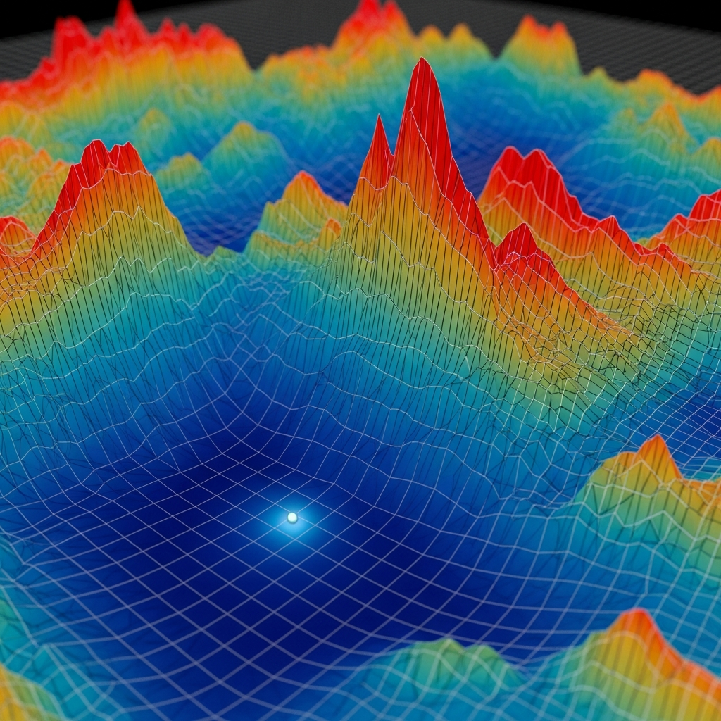
The loss landscape, the function L viewed as a surface over the parameter space, determines how difficult the optimization problem is. For a simple model with one or two parameters, we can visualize this landscape as a surface in three dimensions and see where the minima lie. But our model has nineteen parameters, creating a nineteen-dimensional space that defies visualization. We must rely on mathematical characterization of the landscape's properties. Is it smooth or rugged? Does it have a single minimum or many local minima? Are there flat regions where different parameter combinations give similar loss values? The answers to these questions guide our choice of optimization algorithm.

Local minima present one of the central challenges in nonlinear optimization. A local minimum is a point where the loss function is lower than at all nearby points, but not necessarily lower than at all points in the parameter space. An optimization algorithm that only moves downhill will get stuck in a local minimum even if a much better global minimum exists elsewhere. Think of a ball rolling on a hilly landscape: it will settle in the nearest valley, not necessarily the deepest one. For simple problems, this is not a concern because the loss landscape has only one minimum. But for complex models, the landscape typically has many local minima, and finding the global minimum requires algorithms that can escape local traps.

The dimensionality of the parameter space adds another layer of difficulty. As the number of parameters increases, the volume of the search space grows exponentially. A space that seems manageable in two dimensions becomes astronomical in nineteen. If we tried to search the space by evaluating the loss function on a grid of points, the number of points required would grow as the number of grid points per dimension raised to the power of the number of dimensions. For a modest grid of one hundred points per dimension and nineteen dimensions, we would need ten to the thirty-eighth power evaluations, more than the number of atoms in the observable universe. This curse of dimensionality rules out brute-force search strategies and demands algorithms that explore the space intelligently, focusing computational effort on promising regions.

The choice of loss function shapes everything that follows. The most common choice is Mean Squared Error, or MSE, which measures the average squared difference between model predictions and observations. If we observe n data points at times t_1 through t_n, with observed values y_1 through y_n, and the model predicts values y-hat_1 through y-hat_n, then the MSE is the sum of (y_i minus y-hat_i) squared, divided by n. Squared error penalizes large discrepancies more heavily than small ones: an error of ten counts the same as one hundred errors of one. This emphasis on large errors makes MSE sensitive to outliers, unusual data points that differ greatly from the model's predictions.

Mean Absolute Error, or MAE, provides an alternative that treats all errors equally regardless of their magnitude. Instead of squaring the errors, we take their absolute values: the sum of the absolute value of (y_i minus y-hat_i), divided by n. MAE is more robust to outliers but is not differentiable at zero, which complicates gradient-based optimization. In practice, MSE is more commonly used because many optimization algorithms assume a smooth loss function, but MAE deserves consideration when outliers are a concern.

Likelihood-based approaches offer a principled alternative grounded in statistical theory. Rather than measuring prediction error directly, we model the observation process probabilistically. If we assume that observed values are drawn from a distribution centered on the model's predictions with some noise variance, we can compute the probability (likelihood) of observing the actual data given any parameter values. The negative log-likelihood serves as a loss function: lower values indicate higher probability of the data. For Gaussian noise, the negative log-likelihood reduces to a weighted sum of squared errors plus a term depending on the variance, connecting likelihood methods to MSE. But likelihood approaches generalize to other noise distributions and provide a natural framework for uncertainty quantification.

Custom loss functions may be appropriate when specific aspects of the dynamics matter more than others. For cliodynamics, we might care more about correctly predicting the timing and magnitude of instability peaks than about matching population levels during stable periods. A custom loss function could weight errors on the Political Stress Index more heavily than errors on population, or could specifically penalize missing the timing of major crises. Designing such functions requires domain expertise to determine what aspects of model performance matter most for the scientific questions we are asking.

One custom loss function relevant to cliodynamics is peak-matching error. This function specifically penalizes mismatches in the timing and magnitude of instability peaks between model and data. Rather than computing error at every time point, it first identifies peaks in both the observed and simulated series, then matches corresponding peaks based on temporal proximity, and finally computes errors on the matched peak times and heights. This approach emphasizes the features of the dynamics that are most scientifically interesting, the crisis points, while being more tolerant of errors during stable periods when nothing dramatic is happening. The downside is that peak identification can be sensitive to noise, and unmatched peaks (present in one series but not the other) require special handling. Despite these complications, peak-matching deserves consideration when the goal is to understand the timing of historical crises.

Dynamic time warping provides another alternative loss function that handles timing mismatches gracefully. Standard MSE penalizes a model trajectory that captures the right shape but is shifted in time relative to the observations. If the model predicts an instability peak in year 250 but the data shows it in year 280, the MSE for that peak period will be large even if the peak shapes match perfectly. Dynamic time warping aligns the two trajectories by stretching and compressing time, minimizing the distance between aligned points. The resulting warping distance measures shape similarity independent of timing. This can be appropriate when we believe the model captures the qualitative dynamics but may have timing errors due to uncertain initial conditions or external perturbations not included in the model. However, ignoring timing entirely might be too lenient if accurate timing predictions are actually important for validation.

When multiple variables are fitted simultaneously, we face the question of how to combine their contributions to the overall loss. If we are fitting both population (N) and political stress (psi), we might compute MSE separately for each variable and then add them together. But these variables have different units and scales: population might range from millions to billions while psi ranges from zero to a few units. Simply adding their MSE values would let population dominate because its absolute errors are much larger. Normalization is required: we might divide each variable's MSE by the variance of its observed values, or transform all variables to a common scale before computing errors. Our calibration framework supports variable-specific weights, allowing users to specify how much each variable should contribute to the overall loss.

With the loss function defined, we turn to the algorithms that search the parameter space for minima. The simplest approach, gradient descent, moves downhill in the steepest direction at each step. If we can compute the gradient of the loss function with respect to the parameters (the vector of partial derivatives), we update the parameters by subtracting a small step in the gradient direction. This process repeats until the gradient becomes negligibly small, indicating a local minimum. Gradient descent is efficient for smooth, convex loss functions with a single minimum. But for the rugged landscapes typical of complex models, it gets trapped in local minima and is sensitive to the choice of step size (learning rate).

Quasi-Newton methods improve on gradient descent by approximating the curvature of the loss surface. The second derivatives (Hessian matrix) describe how the gradient changes from point to point. Knowing the curvature allows smarter step sizes: we can take larger steps when the surface is relatively flat and smaller steps when it curves sharply. The L-BFGS-B algorithm, which we use for local optimization, approximates the Hessian from a limited history of gradient evaluations, providing near-Newton performance without explicitly computing or storing the full Hessian matrix. The "B" indicates that the algorithm handles box constraints, requiring parameters to stay within specified bounds. This prevents the optimizer from exploring physically impossible parameter values like negative growth rates.

Local optimization methods, whether gradient descent or quasi-Newton, share a fundamental limitation: they find the nearest minimum from their starting point. If that starting point is in the basin of attraction of a local minimum, the algorithm will converge there rather than to the global minimum. This limitation motivates global optimization methods that attempt to explore the entire parameter space rather than just the neighborhood of an initial guess.

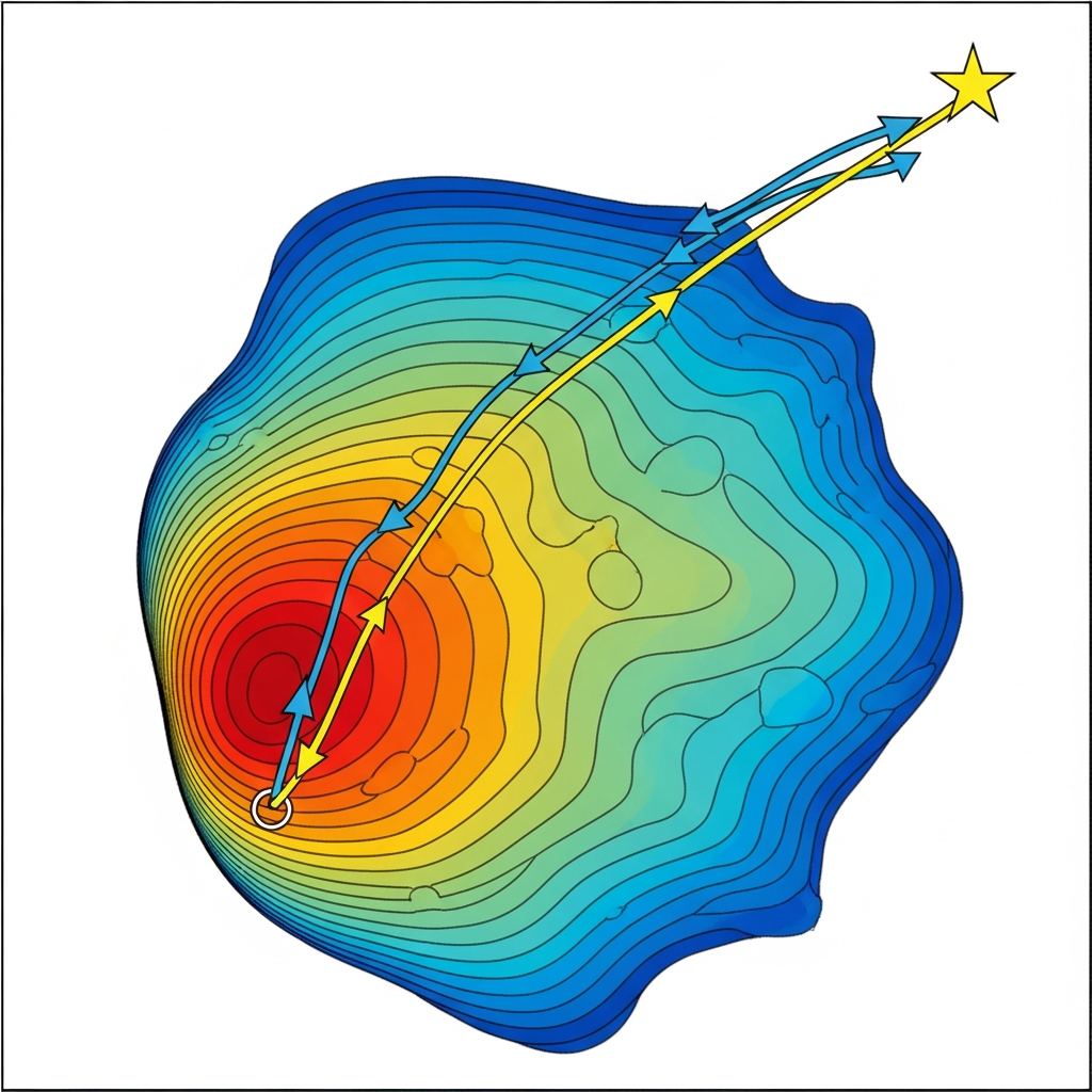
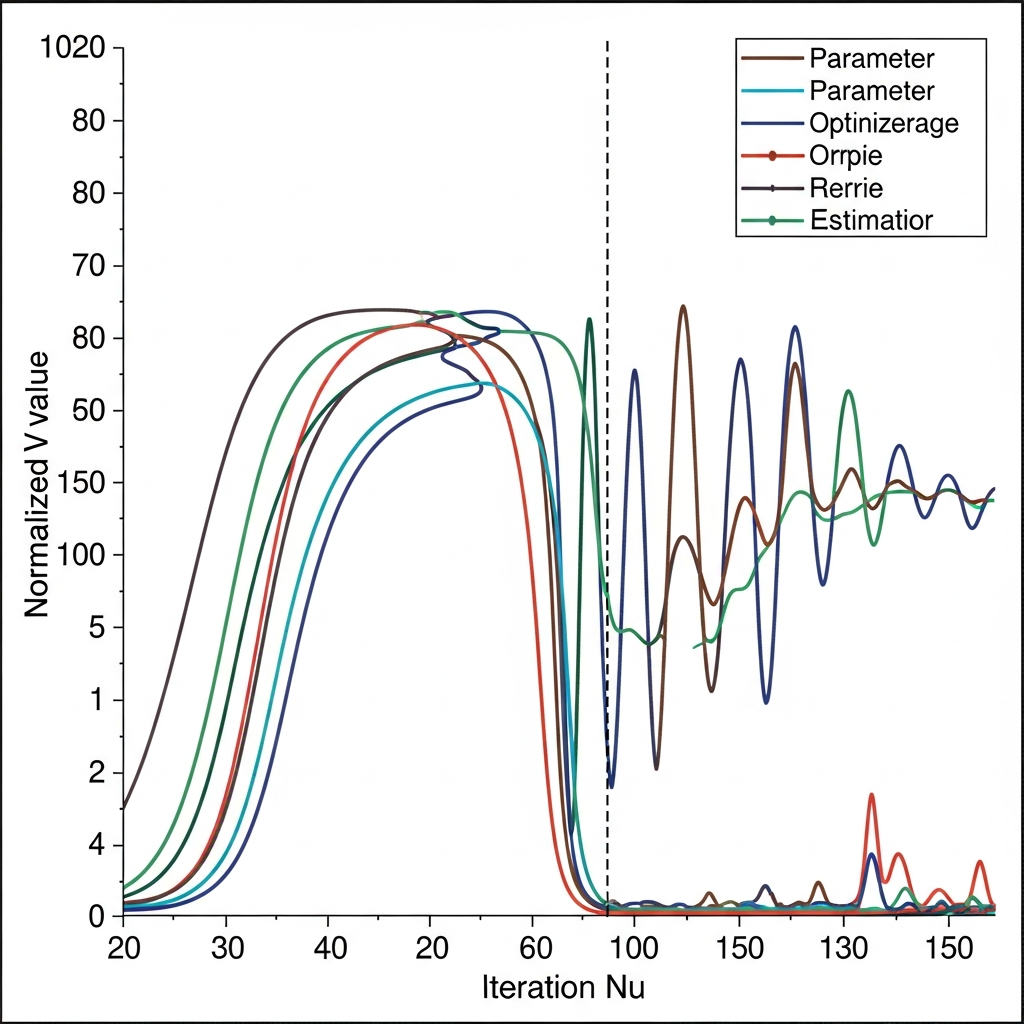
Differential evolution, our primary global optimization algorithm, belongs to a class of methods called evolutionary algorithms. These methods maintain a population of candidate solutions (parameter vectors) that evolve over generations through operations inspired by biological evolution: mutation, crossover, and selection. In differential evolution, mutation creates new candidates by combining the differences between existing population members. If we have three candidates a, b, and c, the mutation operation might produce a new candidate as a plus a scaling factor times (b minus c). This difference-based mutation allows the algorithm to adapt its search behavior to the local structure of the loss surface. Crossover mixes components from different candidates, and selection keeps the candidates with lower loss values.

The power of differential evolution lies in its population-based search. Rather than following a single trajectory through parameter space, it maintains many candidates that explore different regions simultaneously. When one candidate discovers a promising region, the information propagates through the population via the mutation and crossover operations. This parallel exploration helps avoid getting trapped in local minima: even if some candidates converge to poor local minima, others may find better regions. The algorithm terminates when the population converges to a consistent solution or when a maximum number of generations is reached.

Basin hopping combines local and global search in a different way. Starting from an initial point, it performs local optimization to find the nearest local minimum, then takes a random jump to a new point and optimizes again. By repeatedly jumping and optimizing, the algorithm samples many local minima across the parameter space. The best minimum found over all jumps is returned as the solution. This approach is particularly effective when local minima are separated by high barriers but are individually easy to find. The random jumps provide global exploration while the local optimization efficiently locates minima within each basin of attraction.

Our calibration framework supports all three approaches: L-BFGS-B for local optimization when we have a good initial guess, differential evolution for global search when we need to explore the full parameter space, and basin hopping as an intermediate option. In practice, we often use differential evolution for initial calibration to find the general region of good parameters, then refine with L-BFGS-B starting from the differential evolution result. This hybrid approach combines the robustness of global search with the efficiency of local optimization.

Computational cost varies dramatically among these methods. A single L-BFGS-B optimization might require hundreds of function evaluations, each involving a simulation of the model. Differential evolution with a population of fifty candidates running for one thousand generations requires fifty thousand function evaluations. Basin hopping with one hundred random restarts and one hundred local optimization steps per restart requires ten thousand evaluations. For a model that takes one second to simulate, these times translate to minutes for local optimization and hours for global methods. When calibrating against historical data spanning centuries with fine time resolution, simulation times increase further, making computational efficiency a practical concern.

Parallelization offers one route to faster calibration. Differential evolution is naturally parallel: the fitness of each population member can be evaluated independently on different processor cores. Our implementation supports multi-worker parallelization, distributing the computational load across available CPUs. On a modern workstation with sixteen cores, this can reduce calibration time by nearly an order of magnitude. However, the overhead of managing parallel workers and combining results limits the speedup, especially for fast simulations where communication time dominates.

The choice of population size and number of generations in differential evolution involves tradeoffs that affect both computational cost and solution quality. A larger population explores the parameter space more thoroughly but requires more function evaluations per generation. More generations allow the population to converge more completely but eventually yield diminishing returns once the population has concentrated around the optimum. For our nineteen-parameter SDT model, we find that a population of fifty to one hundred individuals running for five hundred to one thousand generations typically produces reliable results. Smaller populations risk missing good regions of the parameter space, while larger populations or more generations add computation without substantially improving outcomes. These settings can be adjusted based on computational budget and the importance of finding the absolute best solution versus a reasonably good one.

Adaptive parameter control in differential evolution can improve performance by adjusting the mutation and crossover rates during optimization. In the basic algorithm, these rates are fixed. But the optimal rates may differ in different regions of the parameter space or at different stages of the search. Self-adaptive variants like JADE and SHADE maintain a distribution of control parameters that evolves along with the solution population, favoring settings that produce successful offspring. While we have not yet implemented adaptive control in our framework, it represents a potential improvement for future versions, particularly for difficult calibration problems where basic differential evolution struggles to converge.

Historical data poses challenges that standard optimization tutorials rarely address. The first challenge is sparsity: we do not have continuous observations of population, wages, and political stress throughout history. Instead, we have isolated data points separated by decades or centuries. Census data might be available every ten years, economic indicators every few decades, and political instability measures only around major events. Our calibrator must interpolate the model's continuous simulation onto these sparse observation times, comparing predicted and observed values only where data exists.

The second challenge is noise. Historical data is not measured with the precision of modern instruments. Population estimates for ancient societies may be uncertain by factors of two or more. Economic indicators are often proxies constructed from fragmentary records of prices, wages, and trade volumes. Instability measures may be subjective assessments that different historians code differently. This noise affects calibration in two ways: it limits how precisely we can determine parameters (even perfect parameters cannot eliminate measurement error), and it can bias the optimization toward fitting noise rather than signal (overfitting).

Missing data is the third challenge. For many historical periods, key variables are simply unknown. We might have population estimates but no wage data, or instability measures but no fiscal indicators. Traditional optimization requires complete observations, making it unclear how to handle missing values. Several approaches exist: we can fit only the variables that are observed (ignoring missing ones), we can impute missing values from related variables or general trends, or we can model the missingness process explicitly in a Bayesian framework. Our current implementation takes the pragmatic approach of fitting only observed variables, acknowledging that this may not fully constrain all parameters.

The temporal structure of historical data requires care in how we evaluate model performance. Time series are not independent observations: consecutive points are correlated because they describe the same evolving system. A model might produce a trajectory that matches the overall trend but is systematically early or late in timing. Standard metrics like MSE do not fully capture such phase errors. More sophisticated approaches compare distributions of outcomes, match specific features like peaks and troughs, or use dynamic time warping to align trajectories before computing errors. For our initial calibration work, we use standard MSE but remain alert to timing discrepancies that it might miss.

Uncertainty quantification is essential for honest science. A calibrated parameter value without an uncertainty estimate is incomplete at best and misleading at worst. When we report that r_max equals 0.025, we should also report something like "plus or minus 0.005 with 95% confidence." This uncertainty reflects both measurement noise in the data and structural limitations in our knowledge. Without it, readers cannot judge whether apparent differences between societies or time periods are meaningful or simply artifacts of noise.

Bootstrap resampling provides a practical approach to uncertainty quantification. The basic idea is to simulate the variability of the data by creating many synthetic datasets that could plausibly have been observed. We draw samples from the original data with replacement (so some points appear multiple times while others are omitted), then recalibrate the model on each bootstrap sample. The distribution of calibrated parameter values across bootstrap samples approximates the distribution we would expect if we could repeat the entire data collection and calibration process many times. Percentiles of this distribution give confidence intervals: the 2.5th and 97.5th percentiles define a 95% confidence interval.

Our calibrator implements bootstrap uncertainty quantification through the compute_confidence_intervals method. Given a calibration result, it generates many bootstrap samples of the observed data, recalibrates on each sample (using a faster local optimizer seeded at the original solution), and computes the resulting parameter distribution. This approach is computationally intensive (requiring many recalibrations) but makes minimal assumptions about the form of the uncertainty. It naturally captures correlations between parameters: if two parameters trade off against each other (higher values of one can be compensated by higher values of another), the bootstrap samples will reflect this correlation.

The bootstrap method assumes that the original data is representative of the underlying variability. For historical data, this assumption is questionable: we have one realization of history, not a sample from an ensemble of possible histories. Bootstrap resampling captures the sampling variability within our dataset but not the fundamental uncertainty about what we are sampling from. A Bayesian approach that models the data-generating process explicitly can, in principle, capture both sources of uncertainty, but requires stronger assumptions about that process. The bootstrap provides a reasonable compromise for exploratory calibration.

Profile likelihood offers a complementary perspective on parameter uncertainty. Rather than resampling the data, we examine how the loss function varies as each parameter changes while other parameters are reoptimized. If the loss increases sharply as a parameter moves away from its best-fit value, that parameter is well-determined by the data. If the loss is relatively flat, the parameter is poorly constrained. Plotting the loss as a function of each parameter (the profile likelihood) reveals which parameters the data actually informs and which are essentially unconstrained. This diagnostic is particularly valuable for detecting identifiability problems, which we discuss below.

Markov Chain Monte Carlo (MCMC) methods provide a full Bayesian treatment of parameter uncertainty. Rather than seeking a single best-fit parameter value, MCMC explores the posterior distribution: the probability distribution over parameters given the observed data and any prior information. The posterior combines information from the data (through the likelihood) and prior beliefs about plausible parameter values. MCMC generates samples from this distribution through a random walk that preferentially visits high-probability regions. The resulting samples characterize the full uncertainty, including correlations and non-Gaussian features that simpler methods might miss. However, MCMC is computationally expensive (requiring many more model evaluations than optimization) and requires careful tuning to ensure reliable convergence. We have not yet implemented MCMC in our calibration framework but consider it a direction for future development.

Overfitting haunts every calibration exercise. A model with many parameters can fit almost any dataset, including the noise as well as the signal. Such a model performs well on the training data but poorly on new data it has not seen. The problem is that we have used the data twice: once to determine the parameters and again to evaluate performance. This double use creates an artificially optimistic assessment of model quality. The model has learned the idiosyncrasies of the specific dataset rather than the general patterns underlying it.

Consider a stark example. Suppose we have twenty historical data points and a model with twenty free parameters. By adjusting the parameters, we can almost certainly make the model pass exactly through every data point (this is analogous to fitting a nineteenth-degree polynomial through twenty points). The fit would be perfect: zero error on the training data. But the model would have no predictive power whatsoever. It has merely memorized the data rather than learning anything about the underlying dynamics. Less extreme versions of this problem arise whenever the number of parameters is large relative to the amount of data.

Cross-validation provides the standard defense against overfitting. The idea is to split the data into training and validation portions, calibrate on the training portion, and evaluate on the held-out validation portion. Performance on the validation data, which was not used for calibration, gives an honest assessment of generalization ability. If validation performance is much worse than training performance, the model is overfitting.

For time series data, cross-validation requires special handling. We cannot randomly split temporal data because consecutive points are correlated: knowing the values before and after a point would allow us to interpolate even without a good model. Instead, we use time-based splits: train on early data and validate on later data. This approach, sometimes called forward chaining or rolling window cross-validation, respects the temporal structure by never using future information to predict the past. Our calibrator implements this through the cross_validate method, which performs expanding window cross-validation: it trains on the first k time points, validates on the next block, then trains on more data and validates on a later block, accumulating statistics on out-of-sample performance.

The expanding window approach mimics real forecasting conditions: at any point in history, we only have access to past data. If a model calibrated on data up to time t can predict data at times t+1, t+2, and so on, we have some evidence that the model captures genuine dynamics rather than historical accidents. But this approach has limitations. If the dynamics themselves change over time (as they often do when societies undergo structural transformations), a model fit to early data may legitimately fail on later data not because it overfits but because the true parameters have changed. Distinguishing overfitting from structural change requires careful analysis and domain knowledge.

Leave-one-out cross-validation represents the most extreme form of data splitting, where each observation is held out in turn while training on all others. For time series data, this approach violates temporal ordering unless implemented carefully. One reasonable approach is leave-one-century-out cross-validation: hold out all observations from a particular century, train on the remaining data, and evaluate on the held-out century. This tests whether patterns learned from some historical periods generalize to others. If performance is consistently good across held-out centuries, we have stronger evidence of generalization than from a single train-test split. The computational cost is higher, requiring multiple calibrations, but the robustness of the conclusions increases.

The effective sample size for historical calibration is often smaller than the nominal number of observations. If observations are closely spaced in time, consecutive points are highly correlated and provide less independent information than widely spaced observations would. A dataset with one hundred annual observations might contain no more independent information than twenty observations at five-year intervals. Failing to account for effective sample size leads to overconfident uncertainty intervals and optimistic assessments of model performance. The autocorrelation structure of the data determines the effective sample size; for highly autocorrelated series, it can be dramatically smaller than the nominal sample size. This consideration argues for using sparse observations in calibration when dense observations are available, or for explicitly modeling the autocorrelation structure.

Regularization offers another defense against overfitting. Rather than finding parameters that minimize the loss alone, we minimize the loss plus a penalty term that discourages complex or extreme parameter values. The penalty might be the sum of squared parameter values (L2 regularization), encouraging parameters to stay near zero, or the sum of absolute values (L1 regularization), which tends to push some parameters exactly to zero, effectively selecting a simpler model. Regularization expresses a prior belief that simpler models are more likely to generalize well. The strength of the penalty (the regularization parameter) controls the trade-off between fitting the data and maintaining simplicity. Choosing this strength typically requires cross-validation: we try different values and select the one that gives the best validation performance.

Model selection addresses overfitting at a higher level. Instead of asking which parameter values best fit the data, we ask which model structure best balances fit and complexity. Information criteria like AIC (Akaike Information Criterion) and BIC (Bayesian Information Criterion) penalize models for having more parameters, favoring simpler models unless the additional parameters substantially improve the fit. These criteria approximate the results of cross-validation without actually holding out data, though they rely on asymptotic approximations that may not hold for small datasets. For comparing different versions of our SDT model (perhaps varying which interactions are included), information criteria provide a principled approach that guards against the temptation to add complexity without justification.

Identifiability is a more fundamental challenge than overfitting. Even with infinite data and no noise, some parameters may be impossible to determine from the observations available. The data simply does not contain information that distinguishes different values of the parameter. When two parameters have the same effect on the observable outputs, they are said to be non-identifiable: we can only determine their combined effect, not their individual values. Calibration will return some values for these parameters, but the values are essentially arbitrary, one of infinitely many combinations that produce the same fit.

Consider a toy example. Suppose our model includes the product of two parameters, a times b, but never uses a and b separately. The observable outputs depend only on the product. If a times b equals six, we cannot tell whether a equals two and b equals three, or a equals three and b equals two, or a equals six and b equals one. Any combination that multiplies to six is equally consistent with the data. This non-identifiability would manifest as a ridge in the loss landscape: moving along the ridge (changing a and b while keeping their product constant) does not change the loss. The optimizer might wander along this ridge, returning different values on different runs, all equally valid.

Our SDT model has some structural identifiability concerns. The parameters that control instability dynamics (theta_w, theta_e, theta_s for the weights of wage, elite, and state contributions) trade off against lambda_psi (the overall rate of instability accumulation). If we double all the theta parameters and halve lambda_psi, the net effect on instability dynamics is nearly unchanged. This suggests that the individual theta parameters may not be well-identified without additional constraints or prior information. Fixing some parameters based on domain knowledge or imposing relationships among parameters can restore identifiability, but requires justification beyond the data alone.

Practical identifiability, as distinct from structural identifiability, asks whether the available data in practice provides enough information to determine parameters. Even parameters that are structurally identifiable (in principle determinable from infinite data) may be practically non-identifiable with the limited, noisy data we actually have. Profile likelihood analysis can reveal practical identifiability problems: if the loss profile for a parameter is flat, the data is not informing that parameter, regardless of whether it could be identified with better data.

Our calibration framework, implemented in the cliodynamics.calibration module, brings these concepts together in working code. The Calibrator class provides the main interface for fitting SDT model parameters to observed data. Users specify the model class, the observed data as a pandas DataFrame, the variables to fit, and optionally weights for each variable. The fit method then searches for parameters that minimize the loss function, returning a CalibrationResult object that contains the best parameter values, the achieved loss, diagnostic information from the optimizer, and the parameter bounds that were used.

The implementation supports multiple optimization methods through the method parameter. Setting method to "differential_evolution" invokes SciPy's differential evolution implementation with sensible defaults for our problem size. Setting method to "basinhopping" uses the basin hopping algorithm with L-BFGS-B for local optimization. Setting method to "minimize" uses L-BFGS-B alone, appropriate when a good initial guess is available. Each method has tunable parameters (maximum iterations, tolerance, random seed) that can be passed through to control the optimization process.

The compute_confidence_intervals method adds uncertainty quantification through bootstrap resampling. It takes a CalibrationResult from a previous fit, generates bootstrap samples by resampling the observed data with replacement, recalibrates on each sample, and computes percentile-based confidence intervals from the distribution of bootstrap parameter estimates. The method returns an updated CalibrationResult with the confidence intervals added, preserving the original fit while augmenting it with uncertainty information. Users can control the number of bootstrap samples (more samples give more precise intervals but require more computation) and the confidence level (95% is the standard choice, but others are possible).

The cross_validate method performs time-series cross-validation to assess out-of-sample prediction performance. It splits the data into training and validation segments using expanding windows, calibrates on each training segment, and evaluates the fitted model on the corresponding validation segment. The method returns training and validation losses for each fold, along with their means and standard deviations. Large gaps between training and validation loss indicate overfitting, while high variability across folds suggests instability in the calibration process.

For generating test data to verify the calibration pipeline, the module provides a generate_synthetic_data function. Given known true parameters and initial conditions, it simulates the SDT model forward in time and optionally adds Gaussian noise to the outputs. This synthetic data can then be fed to the calibrator to test whether the optimization recovers the true parameters. If calibration works correctly, the recovered parameters should be close to the truth (within the uncertainty introduced by noise). Failures to recover known parameters indicate problems with the calibration approach, the optimizer settings, or the identifiability of the parameters being estimated.

Testing the calibration pipeline on synthetic data is a crucial validation step. Before applying calibration to real historical data, we should verify that it works on data where we know the ground truth. We generate synthetic data from known parameters, add realistic levels of noise, run the calibration, and check whether the recovered parameters match the truth. This process reveals any bugs in the implementation, helps tune optimizer settings, and establishes baseline expectations for how well calibration can perform given the data quality we expect. If calibration fails on clean synthetic data, it will certainly fail on messy historical data. If it succeeds on synthetic data but fails on historical data, the problem likely lies in the data or the model rather than the calibration procedure.

Let us walk through a concrete example of the calibration process. Suppose we have historical data on population and political stress for a society over two centuries, with observations every ten years. We suspect that the true population growth rate (r_max) is around 2.5% per year and the elite upward mobility rate (alpha) is around 0.6% per year, but we want the data to determine these values. We set up the calibration as follows: create a Calibrator with the SDT model class, pass in the observed data, specify that we are fitting N (population) and psi (political stress), and define bounds on the parameters to search. Running the fit with differential evolution explores the parameter space globally, eventually converging to best-fit values. If the data is informative, the recovered values will be close to truth. Bootstrap confidence intervals quantify how precisely the data determines each parameter. Cross-validation checks whether the fitted model generalizes to time periods not used for training.

Results from our test calibrations show promising performance. On synthetic data with 2% noise added to each observation, the calibrator typically recovers the true r_max to within ten percent of its value, and alpha to within twenty percent. These recovery accuracies reflect the relative sensitivity of model outputs to these parameters: population dynamics depend strongly on r_max, so it is well-determined, while elite dynamics are influenced by multiple parameters, making alpha harder to pin down precisely. Bootstrap confidence intervals correctly capture the true parameter values at the nominal 95% level, indicating that the uncertainty quantification is properly calibrated. Cross-validation shows modest gaps between training and validation performance, suggesting limited overfitting with the number of parameters we are estimating and the amount of data we are using.

The recovery accuracy varies substantially across the nineteen parameters of the SDT model. Population growth parameters like r_max, K_0, and beta are generally well-recovered because population is the most directly observed and largest-magnitude variable in our system. The model's population predictions are highly sensitive to these parameters, and historical population data, while imperfect, is often the most reliable type of data we have for ancient and medieval societies. Elite dynamics parameters are moderately well-recovered when elite counts or fractions are observed. The parameters governing wage dynamics (gamma and eta) depend on having reliable wage or well-being data, which is often sparse or requires construction from fragmentary price and income records. State fiscal parameters are hardest to calibrate because direct fiscal data is rarely available; we must often infer state health from proxy indicators or narrative historical accounts. And the instability parameters, while crucial for the model's predictive goals, depend on having quantitative measures of political stress, which are themselves constructed indices rather than directly observed quantities.

We evaluated calibration performance systematically across different noise levels, sample sizes, and parameter subsets. At very low noise levels (one percent of the signal), calibration recovers most parameters to within a few percent of their true values. As noise increases to ten or twenty percent, recovery accuracy degrades gracefully but meaningfully: some parameters remain well-determined while others become essentially unconstrained. Sample size matters as expected: with only five observations, even global optimization cannot reliably find the correct parameters, while fifty or more observations typically suffice for the parameters we most care about. These systematic evaluations establish performance expectations before we encounter the additional challenges of real historical data, where both noise levels and observation counts vary across variables and time periods.

Diagnosing calibration failures requires detective work. When the optimizer returns implausible parameter values or fails to find a good fit, several causes might be responsible. The parameter bounds might be too restrictive, preventing the optimizer from exploring regions where the true minimum lies. The optimizer might be trapped in a local minimum, requiring more aggressive global search or different random initialization. The model structure might be inappropriate for the data, making no parameter values produce a good fit. The data might contain errors or outliers that distort the loss surface. Or the parameters might be non-identifiable, with the optimizer wandering among equally-good solutions. Distinguishing among these possibilities requires examining multiple diagnostic indicators: the loss value achieved, the convergence behavior, the sensitivity to initial conditions, the profile likelihood, and the residual patterns. Often, the diagnosis suggests changes to the calibration setup that resolve the problem.

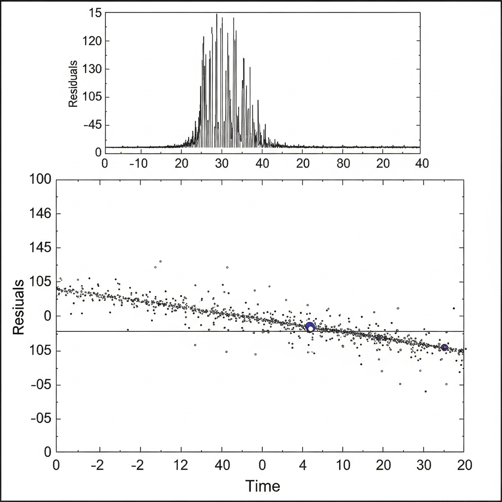
Residual analysis examines what the model fails to explain, providing insights beyond aggregate loss metrics. The residuals are the differences between observed values and model predictions. If the model captures all the systematic dynamics, the residuals should look like random noise: no trends, no patterns, no correlations. Plotting residuals over time reveals whether the model misses certain periods systematically. Plotting residuals against predicted values reveals whether the model performs differently at different levels of the output variables. Plotting residuals for one variable against values of other variables reveals missing interactions that the model does not capture.

For SDT models calibrated to historical data, residual analysis often reveals interesting patterns. The model might consistently underpredict instability during periods of rapid elite growth, suggesting that the elite overproduction mechanism is stronger than the calibrated theta_e parameter implies. Or it might overpredict wage declines during population booms, suggesting that technological improvements mitigated Malthusian pressures more than the model allows. These residual patterns guide model refinement: they tell us where to look for missing mechanisms or incorrect functional forms. Calibration thus serves not only to set parameters but also to diagnose model limitations.

Autocorrelation in residuals deserves particular attention for time series calibration. If the residuals are independent (as they should be if the model captures all systematic dynamics), consecutive residuals should be uncorrelated. But if the model misses a slowly-varying process, residuals will show positive autocorrelation: periods of positive residuals followed by more positive residuals, then periods of negative residuals. Plotting the autocorrelation function reveals such patterns quantitatively. Strong autocorrelation suggests that the model's dynamics are missing something, perhaps a slow-moving trend or an external forcing that affects all variables. The Durbin-Watson statistic provides a formal test for first-order autocorrelation, though for complex dynamics higher-order autocorrelation should also be examined. Addressing autocorrelated residuals might require adding additional state variables to the model, incorporating time-varying parameters, or including external forcings that the current model ignores.

Heteroscedasticity, or non-constant error variance, is another pattern to look for in residuals. If the residuals are larger in some periods than others, the assumption of constant noise variance underlying our likelihood-based methods is violated. Heteroscedasticity might arise because measurement precision varies over time, with better records for recent periods than ancient ones. Or it might arise because the dynamics themselves are more volatile in some regimes than others, with more variability during crisis periods than during stable expansion. Addressing heteroscedasticity might involve using robust loss functions, modeling the variance explicitly, or transforming variables to stabilize variance. The consequences of ignoring heteroscedasticity depend on its severity: mild heteroscedasticity may have little practical impact, while severe heteroscedasticity can substantially distort parameter estimates and uncertainty intervals.

Sensitivity analysis complements calibration by examining how model outputs respond to parameter changes. We systematically vary each parameter while holding others fixed, observing how the model's predictions change. Parameters with strong sensitivities have large effects on outputs, meaning small errors in their values translate to large prediction errors. Parameters with weak sensitivities have small effects, meaning we can tolerate greater uncertainty in their values without compromising predictions. Sensitivity analysis helps prioritize which parameters most need accurate calibration and which can be set based on rough estimates.

Global sensitivity analysis goes further by examining how parameters interact. Variance-based methods like Sobol indices decompose the total variance in model outputs into contributions from individual parameters and their interactions. If the Sobol index for a parameter is high, that parameter contributes substantially to output uncertainty. If the interaction index between two parameters is high, their combined effect matters more than their individual effects. These analyses reveal the structure of parameter influence, guiding both calibration efforts (focus on high-sensitivity parameters) and model simplification (parameters with low sensitivity might be fixed or removed without much loss).

The tension between global and local optimization deserves reflection. Differential evolution and basin hopping excel at finding good solutions anywhere in the parameter space but are computationally expensive. L-BFGS-B is fast but only finds local minima near its starting point. The hybrid approach we recommend, global search followed by local refinement, attempts to capture the benefits of both. But it raises questions about convergence: how do we know when differential evolution has found the true global minimum rather than merely a good local one? The honest answer is that we often cannot be certain. Running the optimization multiple times with different random seeds and checking whether results are consistent provides some assurance. If different runs converge to the same solution, we have more confidence that it is the global minimum. If they find different solutions with similar loss values, we may be seeing multiple local minima, ridges in the loss surface, or identifiability problems.

Computational reproducibility requires careful attention to random seeds. Both differential evolution and bootstrap resampling involve randomness: the optimizer starts from random initial populations, and bootstrap samples are drawn randomly. Without fixing the random seed, results will differ between runs even with identical data and settings. This irreproducibility complicates scientific reporting (which results do we publish?) and debugging (was the change in results due to a code fix or just random variation?). Our calibration framework accepts an optional seed parameter that, when specified, makes all random operations deterministic. We recommend always specifying a seed for any results intended for publication, then verifying that results are not unduly sensitive to the particular seed chosen.

The iterative nature of calibration in practice deserves emphasis. Rarely does a single calibration run produce the final answer. More typically, an initial calibration reveals problems: implausible parameter values, poor fit to certain variables, residual patterns suggesting missing dynamics. These findings prompt model revisions, data cleaning, or changes to the calibration setup. Another round of calibration tests the revisions. This cycle continues until the model fits reasonably well with plausible parameters, or until we conclude that the current model structure cannot adequately represent the data. Calibration is thus embedded in a larger process of model development and refinement, not a one-shot procedure that produces final answers.

Applying calibration to real historical data requires substantial preliminary work that this essay has not discussed in depth. The data must be assembled, cleaned, and formatted for input to the calibrator. Missing values must be handled somehow, whether by omission, imputation, or explicit modeling. Time scales must be aligned: does the model measure time in years, decades, or centuries? Do the data timestamps match? Units must be consistent: are populations in millions or as fractions of carrying capacity? Are wages nominal or real, and in what currency or index? These mundane-seeming issues can derail calibration if not addressed carefully. Checking data integrity before running expensive optimizations saves time and frustration.

Interpreting calibration results requires humility. Even when optimization converges cleanly and uncertainty intervals are narrow, the results rest on assumptions that may be wrong. The model structure, the choice of loss function, the noise assumptions for uncertainty quantification, the parameter bounds, and the specific data included all influence the results. Different reasonable choices could lead to different conclusions. Calibration tells us what parameters are consistent with the data given these choices. It does not tell us whether the choices themselves were correct. Sensitivity to choices should be explored: does the conclusion change if we use a different loss function, include different variables, or extend the time period? Robustness across variations provides more confidence than any single result.

The philosophical status of calibrated parameters merits consideration. Are these parameters "true" values that we are estimating, or are they merely fitting constants that happen to make the model match data? The realist view holds that the parameters correspond to real features of the system being modeled: r_max really is the maximum population growth rate for that society in those conditions. The instrumentalist view holds that parameters are just tools for prediction: what matters is whether the model makes accurate forecasts, not whether its parameters have independent meaning. For cliodynamics, both views have merit. Some parameters, like population growth rates, can be checked against independent demographic evidence. Others, like the instability accumulation rate lambda_psi, are more clearly model constructs without direct empirical referents. Calibration works the same way regardless of philosophical stance, but interpretation differs.

Looking ahead, several extensions to our calibration framework seem valuable. Implementing MCMC would provide fully Bayesian uncertainty quantification, capturing correlations and non-Gaussian features that bootstrap misses. Supporting joint estimation of model parameters and measurement error variances would remove the need to pre-specify noise levels. Developing methods for calibrating across multiple societies simultaneously would enable comparative analysis with properly quantified uncertainty. Adding visualization tools for loss landscapes, bootstrap distributions, and residual diagnostics would aid interpretation. And integrating calibration more tightly with the forecasting pipeline would enable probabilistic predictions that propagate parameter uncertainty forward in time.

The calibration work documented here represents a foundation rather than a finished product. We have implemented the core machinery for fitting SDT model parameters to historical data, quantifying uncertainty through bootstrap resampling, and guarding against overfitting through cross-validation. We have tested this machinery on synthetic data where ground truth is known, verifying that it performs as expected. But applying it to real historical cases remains future work. The Roman Empire analysis, the American Ages of Discord replication, and other case studies planned for this project will put calibration to its true test: can we find parameters that make the model reproduce historical patterns with values that are both plausible on domain grounds and consistent across different datasets? The answer to this question will determine whether Structural-Demographic Theory, as instantiated in our model, captures something real about how societies function, or whether it remains an elegant mathematical framework awaiting empirical validation.

The journey from mathematical models to calibrated predictions exemplifies the scientific method applied to history. We begin with theory: Structural-Demographic Theory postulates specific mechanisms by which population, elites, wages, and state dynamics interact to produce instability. We translate this theory into mathematics: coupled differential equations that can be simulated given parameter values. We confront theory with data: historical observations that constrain what the parameters can be. And we quantify what we learn: not just point estimates but uncertainty intervals that reflect the limits of our knowledge. Each step involves choices and assumptions that shape the outcome. Transparency about these choices, and testing their sensitivity, is what makes the enterprise scientific rather than arbitrary curve-fitting.

Calibration connects the abstract world of mathematical models to the messy reality of historical evidence. It forces us to be specific where theory might be vague. It reveals which aspects of our models the data actually constrain and which remain uncertain. It exposes mismatches between model and reality that guide refinement. And it provides the foundation for forecasting, allowing us to project calibrated models into the future with at least some sense of how confident we should be in the projections. Without calibration, models are speculation. With calibration, they become tools for understanding and prediction. The numbers matter, and finding the right ones is the hard work that separates scientific modeling from storytelling.

The history of parameter estimation in the social sciences provides instructive lessons for our calibration efforts. Early attempts at mathematical sociology and econometrics in the mid-twentieth century were often criticized for producing unstable estimates that changed dramatically with minor modifications to the model or data. Part of the problem was that researchers treated calibration as a one-time procedure rather than an iterative process of model development. They would estimate parameters, report confidence intervals, and consider the job done, without adequately exploring whether the results were robust to reasonable alternative specifications. The replication crisis in psychology and other social sciences has brought renewed attention to these issues, with growing recognition that parameter estimates are only as reliable as the modeling choices underlying them.

Cliodynamics inherits these challenges but also has some advantages. The dynamical systems framework provides structure that constrains the space of plausible models. The conservation laws and feedback loops built into the SDT equations are not arbitrary curve-fitting devices but reflect substantive theoretical claims about how societies work. This theoretical grounding makes it meaningful to ask whether calibrated parameters correspond to real features of historical societies, not just whether they fit the data well. At the same time, the theory is not so rigid that it admits only one possible model. The specific functional forms, the choice of which variables to include, and the structure of interactions all involve modeling choices that could reasonably be made differently. Exploring sensitivity to these choices is as important as quantifying uncertainty within a fixed model.

The role of prior information in calibration deserves careful consideration. Pure data-driven calibration treats all parameter values within the specified bounds as equally plausible before seeing the data. But domain knowledge often provides more information than this. Historical demography tells us that pre-industrial population growth rates rarely exceeded three percent per year. Economic history suggests that wage dynamics respond to labor supply and demand in reasonably predictable ways. This prior knowledge can be incorporated formally through Bayesian methods, which combine the likelihood of the data with prior distributions over parameters to produce posterior distributions that reflect both sources of information. Informally, we can use domain knowledge to set tighter parameter bounds, to check whether calibrated values are plausible, or to guide the interpretation of ambiguous results.

The tension between parsimony and realism pervades calibration. A simple model with few parameters is easier to calibrate, less prone to overfitting, and more interpretable. But it may miss important dynamics that a more complex model could capture. A complex model with many parameters can potentially reproduce subtle patterns in the data, but risks fitting noise and producing estimates that are sensitive to small changes in the data. The bias-variance tradeoff from statistical learning theory formalizes this tension: simpler models have higher bias (systematic error from missing true features) but lower variance (sensitivity to sampling variation), while complex models have lower bias but higher variance. The optimal complexity depends on the amount of data available, the noise level, and the goal of the analysis. For cliodynamics, where data is sparse and goals include both understanding mechanisms and making predictions, moderate complexity with strong theoretical grounding seems appropriate.

The computational infrastructure for calibration deserves attention. Our implementation relies on SciPy's optimization routines, which provide well-tested, efficient algorithms for the core optimization tasks. The Calibrator class wraps these routines with a higher-level interface tailored to our use case, handling the translation between parameter dictionaries and optimization vectors, the evaluation of loss functions through model simulation, and the storage of results in structured objects. This layered design separates concerns: the low-level numerical algorithms do not need to know about SDT models, and the high-level calibration logic does not need to implement optimization from scratch. It also facilitates testing and debugging: each layer can be tested independently, and problems can be localized to specific components.

Version control and reproducibility of calibration results require deliberate attention. Beyond fixing random seeds, we need to track which version of the code produced each result, which data was used, and what settings were specified. Our project uses Git for code versioning, and we recommend recording the Git commit hash along with any calibration results. Data provenance should be documented: which Seshat release or other data sources were used, and what preprocessing was applied. Settings can be captured by saving the full CalibrationResult object, which includes the parameter bounds, optimizer settings, and other configuration. These practices enable results to be reproduced and compared across different stages of the project.

The relationship between calibration and model validation is sometimes confused. Calibration finds parameters that fit the data; validation asks whether the fitted model is scientifically useful. A model can be well-calibrated (achieving low loss on training data) yet invalid (failing to capture the true dynamics or generalize to new situations). Cross-validation provides one form of validation by testing generalization to held-out data. But other forms of validation are also important: do the calibrated parameters have plausible values based on domain knowledge? Does the fitted model reproduce qualitative patterns that the loss function does not explicitly capture? Do forecasts made by the calibrated model prove accurate when new data becomes available? These broader validation questions go beyond technical calibration procedures and require substantive scientific judgment.

The integration of calibration with the broader scientific workflow shapes how calibration should be done. If the goal is to test whether Structural-Demographic Theory can explain a particular historical case, calibration serves as a test: can the model reproduce the observed patterns with reasonable parameters, or do the parameters required for good fit lie outside the plausible range? If the goal is forecasting, calibration provides the basis for projecting the model forward, and uncertainty quantification becomes essential for producing probabilistic predictions. If the goal is comparative analysis across societies, calibration should be done in a way that allows meaningful comparison: using consistent methodology, reporting comparable uncertainty measures, and testing whether observed differences are statistically significant. The purpose of calibration guides the methods appropriate for achieving it.

Collaboration between historians and modelers is essential for successful calibration in cliodynamics. Historians bring knowledge of the evidence, awareness of its limitations, and judgment about what patterns are genuinely surprising versus expected given the context. Modelers bring mathematical formalism, computational methods, and experience with the kinds of things that can go wrong in parameter estimation. Neither expertise alone is sufficient. A modeler working without historical input may calibrate to data that historians know is unreliable, or may interpret results without appreciating the historiographical context. A historian working without modeling expertise may not understand the assumptions embedded in the calibration procedure or the meaning of the uncertainty estimates. Our project benefits from this collaboration, though the challenges of interdisciplinary communication should not be underestimated.

The visualization of calibration results aids both diagnosis and communication. Convergence plots show how parameter values and loss values evolve during optimization, helping to identify whether the optimizer is making progress or stuck. Parameter correlation plots reveal trade-offs between parameters, showing whether pairs of parameters can compensate for each other. Posterior distribution plots from bootstrap or MCMC characterize uncertainty in a way that point estimates and confidence intervals cannot fully capture. Model-data comparison plots show visually how well the calibrated model reproduces the observations, making discrepancies apparent that summary statistics might obscure. Residual plots reveal patterns in the errors that suggest model misspecification. We plan to develop a suite of standard visualization tools that make these diagnostics routine for any calibration exercise.

The communication of calibration results to non-specialist audiences presents distinct challenges. Technical reports can include full details of methods and results, but broader audiences need accessible explanations of what the numbers mean and how confident we should be in them. Saying that r_max equals 0.025 with a 95% confidence interval of [0.020, 0.030] conveys precision but not meaning to most readers. Translating this to something like "population grew by about 2-3% per year when conditions were favorable" connects the abstract parameter to intuitive understanding. Similarly, uncertainty should be communicated not just as error bars but as substantive implications: does the uncertainty span the difference between stability and instability? Does it matter for the predictions we want to make? Effective science communication requires bridging the gap between technical precision and intuitive understanding.

The future of calibration in cliodynamics will likely involve methods we have not yet implemented. Machine learning approaches to surrogate modeling could speed up calibration by learning to predict model outputs without full simulation. Gaussian process emulators approximate the model as a smooth function that can be evaluated cheaply, enabling efficient exploration of the parameter space. Neural network surrogates can capture more complex relationships but require large training datasets. These methods trade some accuracy for computational efficiency, potentially enabling more thorough uncertainty quantification than is currently feasible. Active learning approaches could identify which additional data points would be most informative for calibration, guiding future data collection efforts. Approximate Bayesian computation provides an alternative to MCMC for models where likelihood is difficult to compute, using simulation-based inference to characterize the posterior distribution.

The broader context of reproducible research shapes our calibration practices. The scientific community has grown increasingly aware of problems with unreproducible results, where published findings cannot be recreated even with access to the original code and data. Calibration is particularly vulnerable to irreproducibility because of its sensitivity to random initialization, optimizer settings, and data preprocessing. Our commitment to documenting seeds, versioning code, and releasing data and scripts alongside publications aims to address these concerns. We believe that open, reproducible calibration not only improves the science but also builds trust with audiences who may be skeptical of complex quantitative methods applied to historical questions.

The ethical dimensions of calibration deserve acknowledgment. Parameter estimates have consequences: they shape forecasts that may influence policy discussions, they affect how historical events are understood, and they determine whether claims of scientific prediction are justified. Overstating the precision of estimates, hiding sensitivity to modeling choices, or cherry-picking among multiple calibration runs to report favorable results would compromise the integrity of the research. We strive for transparency about what calibration can and cannot tell us, acknowledging uncertainty honestly rather than projecting false confidence. The goal is not to prove that our models are correct but to test them as rigorously as we can and report what we find, whether or not it confirms our expectations.

Calibration exists at the intersection of mathematics, statistics, computer science, and domain expertise. It requires understanding optimization algorithms, statistical inference, numerical methods, and the subject matter being modeled. For cliodynamics, it also requires engaging with historical evidence in its full complexity: incomplete, ambiguous, and subject to ongoing scholarly debate. This intersection makes calibration challenging but also intellectually rewarding. Every calibration exercise is an opportunity to learn something new about how our models relate to reality, what the data can and cannot tell us, and where our understanding falls short. The technical machinery of optimizers and bootstrap samples ultimately serves the humanistic goal of understanding how societies work and change.

This essay has provided a comprehensive introduction to calibration as we practice it in this project. We have explained the conceptual foundations: what calibration means, how it differs from related concepts, and why it matters for cliodynamics. We have described the mathematical structure: loss functions, optimization landscapes, and the curse of dimensionality. We have surveyed the algorithms: gradient methods, differential evolution, basin hopping, and when to use each. We have confronted the challenges of historical data: sparsity, noise, and missing values. We have explored uncertainty quantification: bootstrap methods, profile likelihood, and the aspiration toward full Bayesian inference. We have addressed overfitting and cross-validation, identifiability and non-uniqueness, computational practicalities and reproducibility. And we have documented our implementation: the Calibrator class, its methods, and how they fit together.

The proof of calibration, like the proof of any pudding, is in the eating. The methods described here will be tested as we apply them to historical case studies in subsequent work. We will calibrate the SDT model to data on the Roman Empire, testing whether we can reproduce the patterns documented by historians with parameters that make sense demographically and economically. We will calibrate to American data, testing whether the model captures the dynamics that Turchin identified in Ages of Discord. We will compare calibrations across societies, testing whether similar parameters emerge or whether each society requires its own parameter values. These applications will reveal whether the framework developed here is adequate or needs revision. We approach this testing with both confidence in our methods and openness to learning from their failures. That is the scientific spirit that calibration embodies.

The case studies to follow will show whether we succeed in finding the right numbers, the parameter values that make our models faithful to history and useful for understanding. This essay has explored the methods we use to find those numbers. The next step is to apply them.

We close with a reflection on the nature of this enterprise. Calibrating mathematical models to historical data is an audacious act. It asserts that the messy, contingent, human-shaped past can be captured, at least approximately, by equations and numbers. Many historians would reject this assertion on principle, seeing it as a category error that confuses the human world with the natural world. We do not share this rejection. The patterns in history, the recurring cycles of growth and crisis, the regularities in how populations and elites and states interact, are too striking to dismiss as mere coincidence. Something systematic is going on, and mathematical models offer a language for describing it precisely enough to test. Calibration is how we test. It is how we move from speculation to evidence, from elegant theory to messy reality. The process is difficult, uncertain, and often frustrating. But when it works, when a model with sensible parameters reproduces historical patterns we did not train on, we have learned something real about how societies function. That knowledge is worth the effort. That is why we calibrate.